Calibrating Agent-Based Models Using Uncertainty Quantification Methods

, , , ,
and
aUniversity of Leeds, United Kingdom; bSchool of Mathematics, University of Leeds, United Kingdom; cUniversity of Glasgow, United Kingdom; dThe James Hutton Institute, United Kingdom; eSchool of Geography, University of Leeds, United Kingdom
Journal of Artificial
Societies and Social Simulation 25 (2) 1
<https://www.jasss.org/25/2/1.html>
DOI: 10.18564/jasss.4791
Received: 19-May-2021 Accepted: 29-Jan-2022 Published: 31-Mar-2022
Abstract
Agent-based models (ABMs) can be found across a number of diverse application areas ranging from simulating consumer behaviour to infectious disease modelling. Part of their popularity is due to their ability to simulate individual behaviours and decisions over space and time. However, whilst there are plentiful examples within the academic literature, these models are only beginning to make an impact within policy areas. Whilst frameworks such as NetLogo make the creation of ABMs relatively easy, a number of key methodological issues, including the quantification of uncertainty, remain. In this paper we draw on state-of-the-art approaches from the fields of uncertainty quantification and model optimisation to describe a novel framework for the calibration of ABMs using History Matching and Approximate Bayesian Computation. The utility of the framework is demonstrated on three example models of increasing complexity: (i) Sugarscape to illustrate the approach on a toy example; (ii) a model of the movement of birds to explore the efficacy of our framework and compare it to alternative calibration approaches and; (iii) the RISC model of farmer decision making to demonstrate its value in a real application. The results highlight the efficiency and accuracy with which this approach can be used to calibrate ABMs. This method can readily be applied to local or national-scale ABMs, such as those linked to the creation or tailoring of key policy decisions.Introduction
Agent-based modelling has grown in popularity over the past twenty years (Heppenstall et al. 2020). Its ability to simulate the unique characteristics and behaviours of individuals makes it a natural metaphor for modelling and understanding the impacts of individual decisions within social and spatial systems. Applications range from creating models of daily mobility (Crols & Malleson 2019), consumer behaviour (Sturley et al. 2018) and infectious disease modelling (Li et al. 2017).
However, there remain important methodological challenges to be resolved if the full potential of agent based modelling is to be realised. The maturation of the agent based modelling approach is reflected in several recent position pieces (Manson et al. 2020; Polhill et al. 2019). These contributions, whilst wide ranging in their perspectives, have a number of common themes including issues such as common practice for creation of rule sets, embedding behaviour, and establishing robust calibration and validation routines.
Within this paper, we focus on developing a more robust approach to the calibration of model parameters within ABMs. Calibration involves running the model with different parameters and testing, for each case, how well the model performs by comparing the output against empirical data. The goal is to find parameter sets that minimise the model’s error and can be used to provide a range of predictions or analyses (Ge et al. 2018; Grimm et al. 2005; Huth & Wissel 1994; Purshouse et al. 2014).
There are three specific problems related to the calibration of ABMs that need to be addressed. First, computational cost: ABMs are often computationally expensive and thus calibration algorithms that require large numbers of model-runs can be infeasible. Finding optimal parameters while minimising the number of model-runs is essential. Second, there are often uncertainties in the real-world process that an ABM is designed to simulate. This can be because any observations taken are inaccurate or because the system is stochastic and, therefore, multiple observations lead to different results. Third, model discrepancy: models will only ever be abstractions of real-world systems, there will always be a degree of error between an optimised model and an observation (Strong et al. 2012).
Addressing these issues requires a different perspective to be taken by agent-based modellers. We present a novel framework that adapts established methods from the field of uncertainty quantification (UQ). We use history matching (HM) (Craig et al. 1997) to quickly rule out implausible models and reduce the size of the parameter space that needs to be searched prior to calibration. This also reduces the computational cost of calibration. To address uncertainties, we identify and quantify the various sources of uncertainty explicitly. The quantified uncertainties are used to measure the implausibility of parameters during HM, and to inform a threshold of acceptable model error during calibration. Finally, to gain a better understanding of model discrepancy, Approximate Bayesian Computation (ABC) is used to provide credible intervals over which the given parameters could have created the observed data (Csilléry et al. 2010; Marin et al. 2012; Sunnåker et al. 2013; Turner & Van Zandt 2012) .
This framework is successfully applied to three models of increasing complexity. First, we use the well documented model ‘Sugarscape’ (Epstein & Axtell 1996) as a toy example to show step-by-step how to apply the framework, highlighting its simplicity and effectiveness. Second, we use a model that simulates the population and social dynamics of territorial birds, which has previously been used in a detailed study of parameter estimation using a variety of methods, including ABC (Thiele et al. 2014). With this model, we highlight the advantages of using our framework over other methods of calibration in the literature. In this case the number of model-runs required for calibration is reduced by approximately half by using HM before ABC, compared to using ABC alone. Finally, we apply our framework to a more complex ABM that simulates the changes in the sizes of cattle farms in Scotland over a period of 13 years (Ge et al. 2018).
The contribution of this paper is a flexible, more efficient and robust approach to ABM calibration through a novel framework based on uncertainty quantification. The code and results are available online at https://github.com/Urban-Analytics/uncertainty.
Background
Uncertainty and agent-based models
Understanding and quantifying sources of uncertainty in the modelling process is essential for successful calibration. Indeed, quantifying uncertainty (Heppenstall et al. 2020) as well as sensitivity analysis, calibration and validation more generally (Crooks et al. 2008; Filatova et al. 2013; Windrum et al. 2007) are seen as ongoing challenges in agent-based modelling.
Fortunately there is a wealth of prior research to draw on; the field of Uncertainty Quantification offers a means of quantifying and characterising uncertainties in models and the real world (Smith 2013). Typically, there are two forms of uncertainty quantification: forward uncertainty propagation investigates the impacts of random inputs on the outputs of a model (i.e., sensitivity analysis), whereas inverse uncertainty quantification is the process of using experimental data (outputs) to learn about the sources of modelling uncertainty (Arendt et al. 2012) (i.e., parameter estimation or calibration). Here we are concerned with the latter. In the context of ABMs, there are several acknowledged sources from which uncertainty can originate and then propagate through the model. These sources include: parameter uncertainty, model discrepancy/uncertainty, ensemble variance, and observation uncertainty (Kennedy & O’Hagan 2001).
Parameter uncertainty can stem from the challenge of choosing which parameters to use (the model may have too few or too many) as well as the values of the parameters themselves. The values may be incorrect because the measuring device is inaccurate, or the parameters may be inherently unknown and cannot be measured directly in physical experiments (Arendt et al. 2012).
A further complication with parameter uncertainty is that of identifiability or equifinality, where the same model outcomes can arise from different sets of parameter values. This problem is prevalent in agent-based modelling due to the large numbers of parameters that often characterise models. This means standard sensitivity analysis—a commonly used means of assessing the impact of parameters on model results—may have limited utility when performed on an ABM because the model may be insensitive to different parameter values (ten Broeke et al. 2016). This also makes model calibration problematic because it might be difficult to rule out implausible parameter combinations at best, or at worst there may be many ‘optimal’ parameter combinations with very different characteristics.
Model discrepancy, also referred to as model uncertainty, is the “difference between the model and the true data-generating mechanism” (Lei et al. 2020). The model design will always be uncertain as it is impossible to have a perfect model of a real-world process. Instead, a simplification must be made that will rely on assumptions and imperfections (e.g., missing information). If model discrepancy is not accounted for in calibration then the estimated parameter, rather than representing physically meaningful quantities, will have values that are “intimately tied to the model used to estimate them” (Lei et al. 2020). A further difficulty is that it can be hard to separate parameter uncertainty from model discrepancy, which exacerbates the identifiability problem (Arendt et al. 2012).
The third form of uncertainty, ensemble variance, refers to the uncertainty that arises naturally with stochastic models. If the model is stochastic, then each time it is run the results will differ. Typically stochastic uncertainty is accounted for by running a model a large numbers of times with the same parameter combinations (an ensemble of model instances) and the variance in the ensemble output provides a quantitative measure of stochastic uncertainty.
Finally observation uncertainty arises due to imperfections in the process of measuring the target system. This is typically the case when either the equipment used to collect observations provides imprecise or noisy data (Fearnhead & Künsch 2018), or in cases when multiple observations differ due to the natural variability of the real world.
Calibration of agent-based models
The quantitative calibration of ABMs can be categorised into two groups: point estimation, and categorical or distributional estimation (Hassan et al. 2013). The former tries to find a single parameter combination that will produce the best fit-to-data, while the latter assigns probabilities to multiple parameter combinations over a range of plausible values. A variety of point estimation methods have been used, including minimum distance (e.g., least squared errors), maximum likelihood estimation (Zhang et al. 2016), simulated annealing (Neri 2018), and evolutionary algorithms (Heppenstall et al. 2007; Moya et al. 2021). Other methods include ordinary and differential equations, and linear regression (Pietzsch et al. 2020).
Examples of categorical or distributional calibration include Pattern Oriented Modelling (POM), HM, Bayesian networks (Abdulkareem et al. 2019) and ABC (van der Vaart et al. 2015). While point estimation methods aim to find a single parameter point with the best fit-to-data, a selection of the best fitting parameters exposes how different mechanisms in the model explain the data (Purshouse et al. 2014). Furthermore, categorical and distributional estimation methods provide additional information on the uncertainty of the parameters and the model outputs.
Pattern Oriented Modelling (POM), also called inverse modelling, is an approach to develop models that will reproduce multiple patterns from various hierarchical levels and different spatial or temporal scales (Grimm et al. 2005). It is both a calibration approach and a design principle for individual or agent-based modelling. Model elements not needed to reproduce the desired patterns are removed or modified during the model development process. An advantage of this is that validation does not solely happen after creation of the model and on one set of final results alone. Instead, it is validated while being built on multiple patterns, which makes the model more robust and credible (Waldrop 2018).
Approximate Bayesian Computation (ABC)
Bayesian approaches have been used to calibrate ABMs (Grazzini et al. 2017). The Bayesian approach to calibration is not new (Kennedy & O’Hagan 2001), but the difficulty in calculating a likelihood function for complex models hinders the use of this approach for models that aren’t entirely based on mathematically tractable probability distributions.
More recently approximate Bayesian computation (ABC) has been proposed which, unlike traditional Bayesian statistics, does not require the calculation of a likelihood function (Turner & Van Zandt 2012). This is useful for ABMs because deriving a likelihood function for this approach is usually infeasible. The goal of ABC differs fundamentally from the simulated minimum difference. ABC does not attempt to find only the single maximum likelihood parameter, but instead estimates a full posterior distribution that quantifies the probability of parameter values across the entire sample space producing the observed data.
ABC involves sampling a set of parameters from a prior distribution and testing if the model error using those parameters is less than a chosen threshold \(\epsilon\). If the error is smaller than \(\epsilon\) then the parameter set is accepted, otherwise it is rejected. Testing a sufficiently large and diverse range of parameters tested facilitates the approximation of the posterior distribution, i.e., the probability of a parameter set given the data. However, sampling the parameter space and running the model for each set of parameters can be time-consuming, particularly if there are many dependent parameters or the model takes a long time to run. Therefore, efficient sampling methods are necessary. Many different ABC algorithms, such as rejection sampling and sequential Monte Carlo, have been applied in the literature, a selected summary of which can be found by Turner & Van Zandt (2012) and Thiele et al. (2014).
History Matching
History matching (HM) is a procedure used to reduce the size of the candidate parameter space (Craig et al. 1997) to those that are plausible. HM has been applied to ABMs in recent literature (Andrianakis et al. 2015; Li et al. 2017; Stavrakas et al. 2019) but, despite its power, use of the method with ABMs remains limited.
HM involves sampling from the parameter space and measuring the implausibility of each sample. The implausibility is defined by the error of the simulation run (with the chosen parameters) and the uncertainties around the model and observation. Each sample is labelled as non-implausible (the model could produce the expected output) or implausible (the model is unlikely to produce the expected output with the chosen parameters). HM is carried out in waves. In each wave, the parameter space is sampled and split into implausible and non-implausible regions. Each subsequent wave samples from the non-implausible region found in the previous wave. Throughout the procedure, the non-implausible region should decrease as the waves narrow towards the best set of parameters.
Note that HM does not make any probabilistic statements (e.g., a likelihood or posterior distribution) about the non-implausible space (Andrianakis et al. 2015). By contrast, Bayesian calibration methods create a posterior probability distribution on the input space and do not discard implausible areas.
Methods
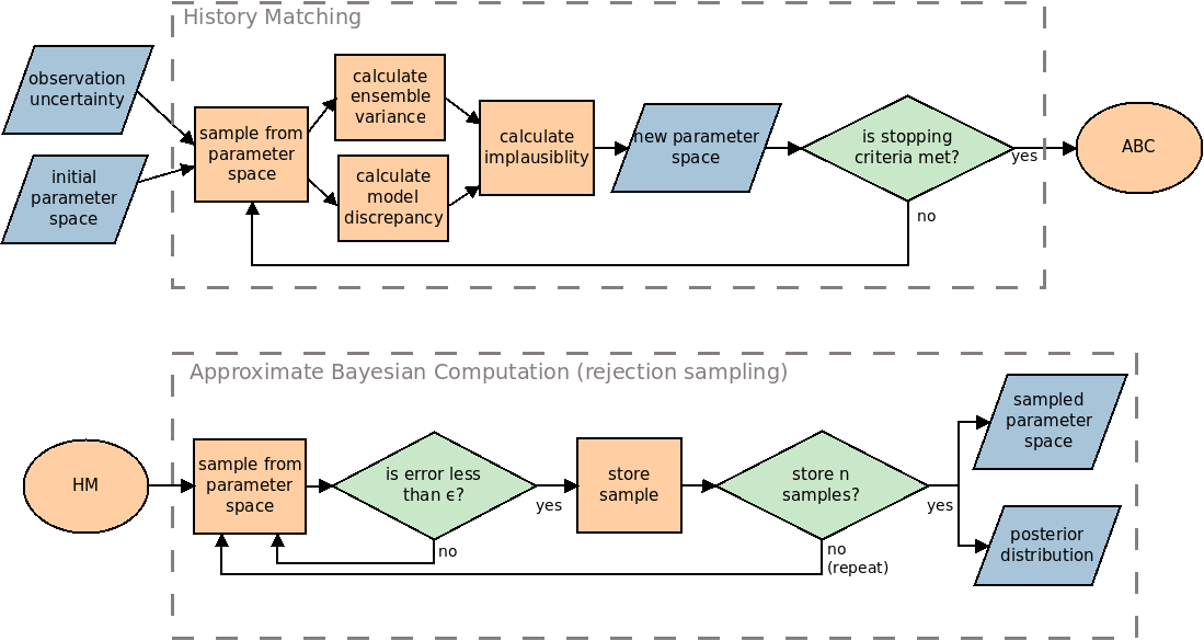
Here, we describe the process of HM, ABC and our framework that combines the two in more detail. Figure 1 highlights the process used. Note that although the diagram describes the rejection sampling method of ABC, any alternative method may be used instead. Whilst HM and ABC are useful when used alone, they become more powerful when used together. Using HM before ABC is advantageous because HM takes uncertainties of the model and observation into account whilst searching the parameter space. This enables the researcher to decide if a parameter may be plausible based on a single run of the model instead of requiring an ensemble of runs for each parameter tested. This allows exploration of the parameter space with fewer runs of the model than with an ABC method alone.
We treat the non-implausible space found through HM as a probabilistic uniform distribution of parameters that fit the model. We propose using this distribution as an informed prior for the ABC procedure, which will then provide a more detailed posterior distribution.
History Matching (HM)
Consider a total of \(R\) observations and \(R\) simulation outputs that are intended to match the observations. Let \(z^r\) be the \(r^\text{th}\) observation, and \(f^r(x)\) be the \(r^\text{th}\) output from the simulator \(f\) with parameters \(x\). For HM, we calculate the implausibility that \(x\) is an acceptable input (i.e., the possibility that the parameter will lead to the expected output). To achieve this, we can compare the model output against the expected output as (Craig et al. 1997):
| \[I^r(x) = \frac{d^2\big(z^r, f^r(x)\big)}{V^r_o + V^r_s + V^r_m}, \] | \[(1)\] |
Ensemble variability is sometimes assumed to be independent of the inputs (Papadelis & Flamos 2019), and so only one possible input (or input vector) is tested. However, ensemble variability may actually differ depending on the input tested and, therefore, it is important to test a small selection of possible inputs in the non-implausible space (Andrianakis et al. 2015).
We use a constant threshold, denoted \(c\), to determine if \(x\) is implausible or otherwise according to the implausbility score \(I^r(x)\) given by Equation 1. If \(I^r(x) \geq c\) then the error between the simulation output and observation is considered too great, even when considering all of the associated uncertainties. If \(I^r(x) < c\), then \(x\) is retained as part of the non-implausible space. The value of \(c\) is usually chosen using Pukelsheim’s \(3\sigma\) rule (Pukelsheim 1994). This implies that the correct set of parameters \(x\) will result in \(I^r(x) < 3\) with a probability of at least 0.95. This process is repeated for multiple points \(x\) within the sample space, discarding those values of \(x\) that are deemed implausible and retaining those that are not implausible. The retained values are then explored in the next wave. For each subsequent wave we must:
- Re-sample within the space that was found to be non-implausible.
- Re-calculate the model discrepancy and ensemble variance. This is necessary because our search space has narrowed towards models that fit better and so it is expected that the uncertainties about this new space will also reduce.
- Perform a new wave of HM within the narrowed space using its newly quantified uncertainties.
The HM process continues until one or more stopping criteria are met (Andrianakis et al. 2015). For example, it may be stopped when all of the parameters are found to be non-implausible. Other common criteria are when the uncertainty in the emulator is smaller than the other uncertainties, or if the output from the simulator is considered to be close enough to the observation. In our examples, we stop the process when either all of the parameters are found to be non-implausible, or the area of the non-implausible space does not decrease (even if some parameters within the area are found to be implausible).
Approximate Bayesian Computation (ABC)
We now describe the process of the rejection sampling ABC algorithm, which we use in our examples. Note, however, that alternative ABC methods that search the sample space more efficiently may be used, such as Markov chain Monte Carlo or sequential Monte Carlo (Thiele et al. 2014; Turner & Van Zandt 2012). To conduct ABC, samples are selected from a prior distribution. As HM does not tell us if any parameter set is more or less probable than another, our prior is represented as a uniform distribution. We use \(n\) particles that search the non-implausible parameter space. Large values of \(n\) (above \(10,000\)) will provide accurate results, whereas a smaller \(n\) may be used at the expense of decreasing the power of the result. For each particle, we sample from our prior and run the model. If the error of the model output is less than \(\epsilon\) we keep the sample for that particle. Otherwise, if the error is too large then we re-sample from the prior until we find a successful parameter set for that particle.
Choosing an optimum value for \(\epsilon\) can be challenging. Setting \(\epsilon\) close to zero would ensure a near exact posterior, but will result in nearly all samples being rejected, making the procedure computationally expensive (Sunnåker et al. 2013). Increasing \(\epsilon\) allows more parameters to be accepted but may introduce bias (Beaumont et al. 2002). One common method to deal with this is to choose a large value in the initial run of the algorithm and gradually decrease \(\epsilon\) over subsequent runs. In this case, each value of \(\epsilon\) may be set ahead of time (Toni et al. 2009) or may be adapted after each iteration (Daly et al. 2017; Del Moral et al. 2012; Lenormand et al. 2013). In our case, we propose using the uncertainties quantified in the final wave of HM to inform the initial choice of \(\epsilon\) and then adapting the value in any further iterations.
Once each particle has a successful parameter set, the posterior distribution can be estimated. Kernel density estimation is a common approach to approximate the posterior (Beaumont et al. 2002). The posterior may then be further refined by re-running the ABC process using the posterior from the first run as the prior for the second run.
A framework for robust validation: SugarScape example
In this paper, we propose using HM together with ABC to calibrate the structure and parameters of an ABM. Specifically, the proposed process consists of the following four steps:
- Define the parameter space to be explored.
- Quantify all uncertainties in the model and observation.
- Run HM on the parameter space.
- Run ABC, using the HM results as a prior.
From these steps, we gain a posterior distribution of the parameters, which can be sampled to obtain a distribution of plausible outcomes from the model. The uncertainties quantified in the second step can then be used to understand the reliability of the model’s outputs.
In this section, we describe the process of these steps for the general case. We then demonstrate each step using the toy model SugarScape (Epstein & Axtell 1996).
Define the parameter space to be explored
We must first decide the ranges that each parameter could take (i.e., the parameter space to be explored). This may be decided qualitatively, through expert judgement (Cooke & Goossens 2008; Zoellner et al. 2019). In some cases, the potential values of a parameter are directly measurable (e.g., the walking speed of pedestrians) and, therefore, quantitative measurements can be used to choose an appropriate range of values for the parameter.
Quantify all uncertainties in the model and observation
Model discrepancy. When searching the parameter space of a model, we estimate the model discrepancy by taking a subset of the samples that are tested for implausibility, ensuring the subset covers the parameter space well (i.e., samples are not clustered together). The model is run once for each sample and the variance of the errors across the samples is calculated as:
| \[V^r_m = \frac{1}{N-1} \sum^N_{n=1} \Big( d\big(z^r, f^r(x_n)\big) - E^r(x) \Big)^2, \] | \[(2)\] |
We measure the error of multiple samples (instead of using only a single sample) because different samples within the space will likely result in different quantified errors, and the variance of different samples should provide a better overview of the whole space than a single sample.
Ensemble variance. We select a subset of \(N\) samples that will be tested as part of HM. For each sample, run the model \(K\) times; larger values of \(K\) will result in a more accurate result at the expense of increasing computational time. The variance is calculated between the \(K\) runs, and the average variance across the \(N\) samples is calculated. Specifically, we measure:
| \[V^r_s = \frac{1}{N} \sum^N_{n=1} \bigg[ \frac{1}{K-1} \sum^K_{k=1} \Big( d\big(z^r, f^r_k(x_n) \big) - E_K^r(x_n) \Big)^2 \bigg], \] | \[(3)\] |
| \[E_K^r(x_n) = \frac{1}{K} \sum^K_{k=1} d\big(z^r, f^r_k(x_n)\big). \] | \[(4)\] |
Observation uncertainty. How observation uncertainty can be measured depends on how the observations are obtained. If the real world process is directly measurable then multiple direct observations can be made and their variance can be used to quantify the uncertainty.
It may also be the case that only indirect measurements can be obtained, and so there will be uncertainty in transforming them so that they can be compared against the model output (Vernon et al. 2010). If an observation cannot be measured, expert judgments may be useful in determining the expected model output and the uncertainty around the expected output. For example, experts may provide quantiles of the expected output, from which uncertainty can be understood (O’Hagan et al. 2006).
Run HM on the parameter space
Given the defined parameter space (in step 1) and the uncertainties quantified (in step 2), we next apply HM. In large or continuous parameter spaces, we use Latin-Hypercube Sampling (LHS) to select samples.
Run ABC, using the HM results as a uniform prior
The final non-implausible space found through HM is used as a uniform prior for ABC. Any appropriate ABC method may be used, such as rejection sampling or sequential Monte Carlo. We propose using the uncertainties measured in the final wave of HM to inform the initial value of \(\epsilon\). Based on Equation 1, let:
| \[\epsilon = 3(V^r_o + V^r_s + V^r_m).\] | \[(5)\] |
The result of performing ABC is a posterior distribution over the non-implausible parameter space identified by HM. Note that we do not perform ABC on the full initial parameter space chosen in step 1.
A Step-by-Step Example: SugarScape
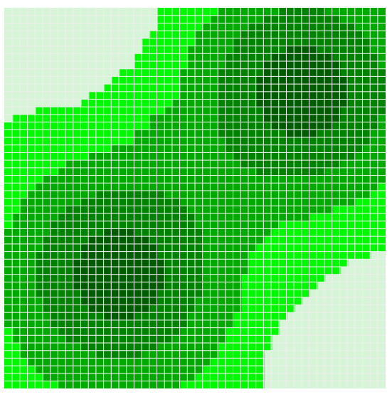
In this section, we provide a step-by-step example of the proposed framework using the Sugarscape model (Epstein & Axtell 1996). Sugarscape is an environment that contains a resource (sugar) and agents that collect and metabolise this resource. The environment is a grid in which sugar is distributed such that some regions are rich with sugar, whilst others are scarce or bare. Figure 2 shows the environment where darker regions indicate higher amounts of sugar. The amount of sugar in a given location is an integer in the range \([0,4]\). At the start of the simulation, 100 agents are placed in a random location of the environment. We use the Sugarscape example provided by the Python-Mesa toolkit by Kazil et al. (2020). This implements a simple version of the model, in which each agents’ only goal is to search for sugar to stay alive. We made minor changes to the code (detailed in our source code) enabling us to change the maximum vision and metabolism of the agents).
In each time step, the agents move, collect sugar, and consume sugar. More specifically, the agent movement rule is (Epstein & Axtell 1996):
- Observe all neighbours within vision range in the von Neumann neighbourhood.
- Identify the unoccupied locations that have the most sugar.
- If multiple locations have the same amount of sugar choose the closest.
- If multiple locations have the same amount of sugar and are equally close, randomly choose one.
- Move to the chosen location.
- Collect all of the sugar at the new location.
- Eat the amount of sugar required to survive (according to the agent’s metabolism).
- If the agent does not have enough sugar, they die.
In each time step, the sugar grows back according to the sugar grow-back rule:
- Increase sugar amount by one if not at the maximum capacity of the given space.
In this example, there are two parameters that we wish to explore. These are:
- The maximum possible metabolism of an agent
- The maximum possible vision of an agent
where metabolism defines how much an agent needs to eat in each step of the model, and vision defines how far an agent can see and, consequently, how far they can travel in each step. Both of these parameters take integer values, and the minimum metabolism or vision an agent may have is 1. The metabolism and vision given to an agent is a random integer between 1 and the calibrated maximum.
The simulation begins with 100 agents. However, some do not survive as there is not sufficient food. As such, our measured outcome is the size of the population that the model can sustain. We create observational data using the output of an identical twin model (a model run to gain an artificial real-world observation). With the maximum metabolism as 4 and the maximum vision as 6, the model was able to sustain a population of 66 agents.
Stochasticity in the model arises from several sources. The initial locations of the agents are chosen randomly in each run. When moving, if multiple locations are equally fit for an agent to move to, the location the agent chooses out of these will be random. The metabolism and vision of each agent is an integer randomly chosen within the defined range. These random choices leads to a stochastic model that will produce different results with each run.
Define the parameter space to be explored
We choose the plausible values for maximum metabolism to be in the range \([1,4]\). We choose 4 as the maximum as there is no location in Sugarscape that has more than 4 sugar. We choose the values for maximum vision to be in the range \([1,16]\). We choose 16 as the maximum as this is the furthest distance from an empty location (i.e., with no food) to a non-empty location.
Quantify all uncertainties in the model and observation
Model discrepancy
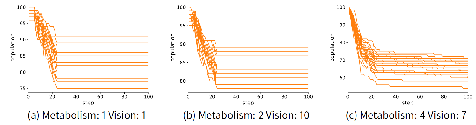
We are interested in finding the parameters that lead to a model that sustains a population of 66 agents. To test this, we ran the model with three different parameter sets over 100 model steps. We repeated this for a total of 30 times to take into account ensemble uncertainty. The parameters are where {metabolism, vision} is {1,1}, {2, 10} and {4, 7}. For each case, we find that in all runs the agent population is stable by step 30 (see Figure 3). To quantify the error of the model, we measure the absolute difference between the population at step 30 and the expected population observed (i.e., 66). Therefore, to measure model discrepancy, we use Equation 2 where \(z=66\) and \(d\big(z, f(x_n)\big) = |z - f(x_n)|\) (note that we have only one measured output and observation in Sugarscape so we omit \(r\) from the formulae).
Ensemble variance
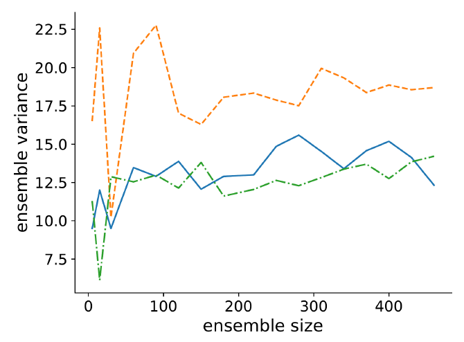
We tested changes in ensemble variance across increasing ensemble sizes to find an optimal size. We tested ensemble variance for the same three parameter sets used to determine when the model has stabilised. These are where {metabolism, vision} is {1,1}, {2, 10} and {4, 7}. Figure 4 shows how the ensemble variance changes with ensemble size. We find the variance stabilised after approximately 200 runs, and so use this as our ensemble size. The measured variance at these points where {metabolism, vision} is {1,1} is 13.0, for {2, 10} is 12.05, and for {4, 7} is 18.34.
Observation uncertainty
As Sugarscape is a toy model, we have no uncertainty in our observation and consequently \(V_o = 0\) in Equation 1.
Run HM on the parameter space
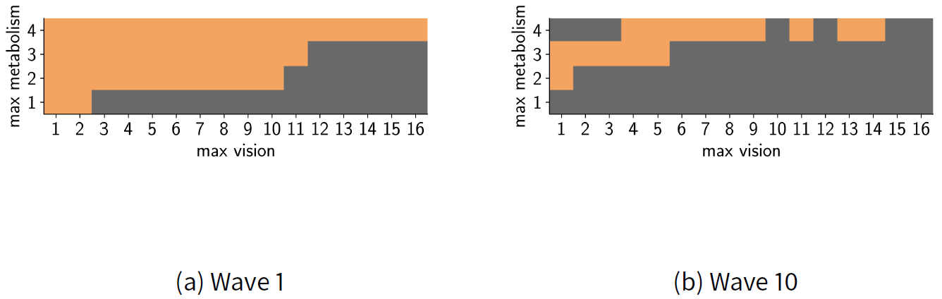
As we have a reasonably small sample space, we measure the implausibility of each parameter pair. Note that typically the sample space is too large and, as described above, LHS sampling is used instead. We performed 10 waves of HM. Wave 10 did not reduce the non-implausible parameter space further so the procedure was stopped. Figure 5 shows the results of the first and final waves, where dark grey represents implausible regions and light orange represents non-implausible regions. The figure shows the whole space explored; that is, prior to wave 1 the full set of a parameters is assumed to be non-implausible (and would be pictured entirely orange), and each set of parameters in the space was tested for implausibility.
In each wave, we retested each of the parameters that were found to be non-implausible in the previous wave. For example, Figure 5 shows the results of the sample space at the end of wave 1. The non-implausible (orange) space here was used as the input for wave 2. In this example, the same parameters were retested because the parameter space is discrete and so there were no other values to test. However, in a continuous space (demonstrated later), new values within the plausible region are typically tested instead of retesting the same values (Andrianakis et al. 2015).
Run ABC, using the HM results as a uniform prior
For Sugarscape, Figure 6 shows the results of the ABC rejection sampling method. The results show that the parameters with the highest probability of matching the observation (i.e., sustaining a population of 66 agents) are where {metabolism, vision} are {4, 7}, with the true parameters {4, 6} (used to create the observation) also obtaining a similarly high probability.
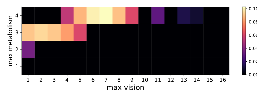
This example illustrates how HM can successfully reduce the space of possible parameter values and ABC can quantify the probability that these non-implausible parameter values could have produced the observed data.
Experiments and Results
In this section, we apply our HM and ABC framework to two ABMs of real-world processes. The first model simulates the movement of territorial birds (Thiele et al. 2014). This model was chosen because many traditional calibration methods have been demonstrated using this model, enabling us to compare our approach with a range of commonly used alternative approaches. The second model is more complex, simulating changes in Scottish cattle farms from external policies over time (Ge et al. 2018). This model was chosen because (i) it provides a real-world test for the proposed framework and (ii) the calibration results themselves can provide interesting insight into the behaviour of the real system.
Case Study 1: Comparing against alternative calibration methods
We now compare our proposed approach to alternative calibration methods, including point-estimation methods (such as simulated annealing) and distribution-estimation methods (such as ABC alone, without HM).
Overview of the model
We use an example model by Railsback & Grimm (2019). The purpose of this model to explore the social groups that occur as a result of birds scouting for new territories. The entities of the model are birds and territories that they may occupy. There are 25 locations arranged in a one-dimensional row that wraps as a ring. Each step of the model represents one month in time, and the simulation runs for 22 years, the first two of which are ignored for the results. In each step, ‘non-alpha’ birds will decide whether to scout for an alpha-bird free location where they can become an alpha-bird. A full ODD of the model used, as well as a link to the source code, is provided by Thiele et al. (2014).
Two model parameters are considered for calibration. These are the probability that a non-alpha bird will explore new locations, and the probability that it will survive the exploration. These are described as the scouting probability and survival probability, respectively. Calibration of the model involves finding values for these two parameters that enable the model to fit three criteria. Measured over a period of 20 years, the criteria are: 1) the average total number of birds, 2) the standard deviation of total birds, and 3) the average number of locations that lack an alpha bird. More details on the model and fitting criteria are provided by Railsback & Grimm (2019) and Thiele et al. (2014). Priors of the parameters are uniformly distributed in the ranges
- Scouting probability: \([0, 0.5]\), and
- Survival probability: \([0.95, 1]\).
Uncertainties in the model
The model aims to match the three criteria above, based on observational data. These criteria are combined to obtain a single measurement of error (therefore only one model output) as provided by (Railsback & Grimm 2019). Specifically, we measure:
| \[d^2(z, f(x)) = e(f(x)^1, z^1) + e(f(x)^2, z^2) + e(f(x)^3, z^3), \] | \[(6)\] |
| \[e(f^r(x), z^r) = \begin{cases} 0 & f^r(x) \in z^r \\ \Big(\frac{\bar{z}^1 - f^r(x)}{\bar{z}^r}\Big)^2 & \text{otherwise}, \end{cases}\] | \[(7)\] |
Observations. The observation variance is captured as a range of values each output can fall within. Instead of treating this variance separately (within \(V_o\) in Equation 1), it is handled when measuring model error in Equation 6.
Model discrepancy. To measure model discrepancy, we select a random sample of 50 parameter sets using an LHS design. We then measure the model discrepancy using Equation 2 with the model error given in Equation 6.
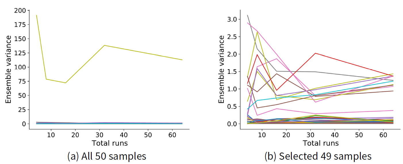
Ensemble variance. We measure ensemble variance as given in Equations 3 and 4. To choose the size of an ensemble we selected 50 samples using an LHS design and ran the model for each sample across a variety of ensemble sizes, measuring the variance for each case. Figure 7 shows the resulting ensemble variance as the total runs of the model within an ensemble is increased. Figure 7 a shows that one sample stands out having a much higher ensemble variance compared to the remaining 49 samples, which are indistinguishable from each other in the figure. Figure 7 b shows the ensemble variance for these remaining 49 samples. The variance appears to stabilise after about 30 runs, so we choose this as our ensemble size.
Results
We use LHS to generate 50 samples within the initial plausible space (this is the same number of LHS samples as used by Thiele et al. 2014).
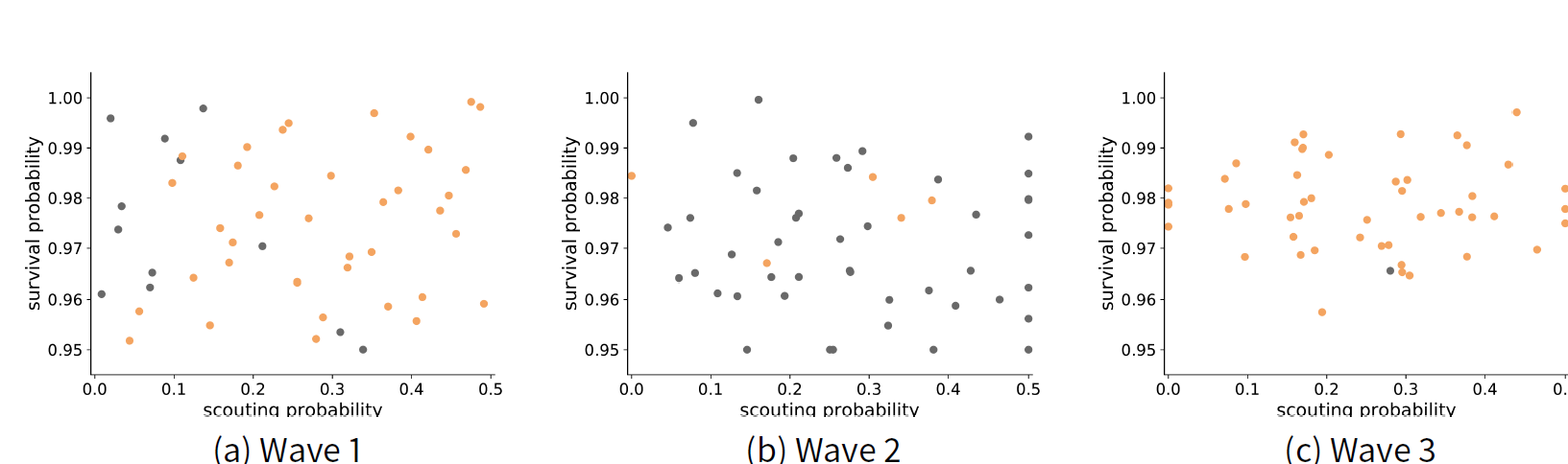
In the first wave, the HM procedure judged that 18 of these 50 samples are non-implausible. We then re-sampled (using a new set of 50 samples) within the new non-implausible region. After the third wave of this procedure, HM was unable to decrease the area of non-implausible space any further.
Figure 8 shows the results of each wave. Each point represents an explored parameter that was found to be implausible (grey) or non-implausible (orange). The results show that the model is more sensitive to scouting survival than to scouting probability. The range of plausible values for scouting survival has reduced to \([0.9606, 0.9925]\), whereas the range of plausible values for scouting probability remains at \([0, 0.5]\). These results are similar to those found with ABC methods by (Thiele et al. 2014).
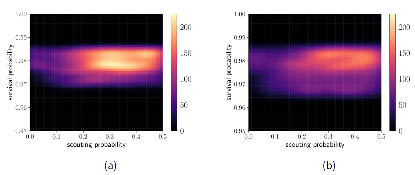
Next, we use the ABC rejection sampling method with 1000 particles to obtain a probability distribution within the sample space. Our prior is a uniform distribution of the non-implausible space found by HM. Figure 9 a shows the resulting posterior distribution, where lighter shades indicate a higher probability. The results show the model is able to match the criteria best if the scouting probability is in the approximate range \([0.2, 0.5]\) and if survival probability is approximately \(0.98\). By contrast, we also performed ABC with the same number of particles but without the HM-informed prior. Figure 9 b shows that the posterior is much broader when information from HM is not used. The results of ABC alone in Figure 9 b is not much more informative than the results from HM alone in Figure 8. These results are similar to those found using ABC alone (Thiele et al. 2014).
We achieved a posterior with 3185 runs of the model using HM and ABC. By contrast, Thiele et al. (2014) obtained similar results with ABC alone using over 11,000 runs. They also demonstrate that simulated annealing and evolutionary algorithms can be used to explore the parameter space. While these methods require fewer runs of the model (256 and 290, respectively) than HM alone (420), they are intended to only provide the best fitting parameters that were tested, whilst HM has the advantage of discovering a region of parameters that fits well and ABC provides a posterior distribution within this region. Note that fewer runs may be used to estimate the ensemble variance, therefore making HM computationally faster, but this may decrease its accuracy and lead to non-implausible samples being quantified as implausible.
Testing the accuracy of the proposed approach
To test the accuracy of our proposed approach of using HM followed by ABC, we compare results from this approach against using ABC alone across a range of parameter values. To do this, we generated 100 pseudo-random pairs of the survival probability and scouting probability parameters. The values were chosen using an LHS design to ensure the samples effectively cover the sample space. For each parameter pair, we want to use the model to produce synthetic data that we then use to calibrate the model. In the previous sections, we calibrated the model using the acceptable ranges of model outputs described in paragraph 5.4, which derived from observational studies. We have seen in Figure 9 that a relatively small range of scouting and survival probabilities are likely to fall within these criteria. Since we are now using the model to produce ‘ground truth’ data over a range of parameter values, we need to identify corresponding ranges of outputs that are acceptable. Thus for each parameter pair, we ran the model 10 times to produce 10 observations, then we set the acceptable range of each of the model fitting criteria to be the corresponding minimum and maximum from the 10 observations. Using these observational ranges, we then performed HM followed by ABC rejection sampling using the same process as described in the previous section (i.e., using Equation 6 to measure error, a total of 30 model runs to measure ensemble variance, a total of 50 samples across the plausible space for each wave of HM, and 1000 samples for ABC rejection sampling). This was carried out for each of the 100 parameter pairs.
Across the 100 parameter pair tests, there were nine examples where the model output total vacant locations (see criteria 3 in paragraph 5.4) was 0 when the model was run to generate observational data. This occurred when the input survival probability was close to 1. The measurement error used by Thiele et al. (2014) is not fit for this situation (resulting in division by zero) and so HM (or any form of calibration) was unable to be performed against these observations. In the 91 remaining tests, HM retained the correct parameters in 90 cases and failed in one case where the expected value for scouting probability was not found. However, in all other tests the plausible range of scouting probability contained the correct test value.1 On average, the non-implausible space for scouting probability was reduced to 88% of its original size, and the space for survival probability was reduced to 42% of its original size.
We next performed ABC rejection sampling with 1000 particles on the 91 cases where HM could be run. We wish to compare the results of using HM before ABC against using ABC alone. Therefore, we run ABC once using the non-implausible space found through HM as an informed prior, and once using an uninformed prior. We found that, on average, ABC required 2047 more model-runs when given an uninformed prior compared to when given the HM-informed prior. The HM procedure required between 80 and 320 runs. Taking this into account, if we subtract the total model runs used to carry out HM from the total runs saved in the ABC process by using the HM-informed prior for each of the 91 tests, then we find we saved an average of 1579 total model runs by using HM before ABC, compared to not using HM. If more particles are used to generate a more accurate posterior this difference is likely to increase.
We analysed the results by measuring the percentage of times the expected value was within the 95% credible interval (CI) across the 91 tests for both scouting probability and survival probability. We also measured the average mean absolute error (MAE) and size of the 95% CI across all tests. Table 1 shows the results. The results indicate that combining HM with ABC produces slightly smaller MAEs and slightly narrower CIs compared with using ABC alone. However, the true parameter is less often contained within the 95% CI. Therefore, using HM with ABC provides results that are more precise (as shown by the smaller MAEs) and more efficient (requiring fewer model runs), but at the cost of CIs that may be too small.
| Contained within 95% CI | Mean Absolute Error | Size of 95% CI | |
|---|---|---|---|
| ABC | |||
| scouting prob. | 92.31 | 0.132 | 0.447 |
| survival prob. | 96.70 | 0.004 | 0.021 |
| ABC and HM | |||
| scouting prob. | 90.11 | 0.130 | 0.434 |
| survival prob. | 93.41 | 0.003 | 0.015 |
Case Study 2: Trends in Scottish Cattle Farms
In this section, we demonstrate that this framework is well suited for Pattern-Oriented Modelling (POM). In POM, patterns are observed within the system being modelled. The structure of the ABM is then designed to explain these observed patterns (Grimm et al. 2005). Multiple plausible models are tested, and those which recreate the observed patterns are retained (Rouchier et al. 2001). We use HM to explore different potential models and rule out those that are implausible (i.e., could not recreate the data even when uncertainties about the model and observed patterns are taken into account). Following HM, we use ABC to calculate the probabilities that the remaining models can recreate the observations.
Overview of the model
Ge et al. (2018) developed a Rural Industries Supply Chain (RISC) ABM that simulates changes in the size of cattle farms over time in Scotland, UK, where size is based on the total number of cattle. The purpose of the model is to explain the phenomenon of farm size polarisation (the trend of disappearing medium-size farms), and predict changes in farm sizes caused by different possible scenarios that could occur as a result of the United Kingdom leaving the European Union. The entities are agriculture holdings that farm cattle. Each step represents one year and the simulation is run for 13 years. The full ODD of the model is provided by Ge et al. (2018).
The model simulates changes in cattle farms over a historic period of 13 years, from 2000 to 2012. The empirical data for this period was collected through an annual survey. Farms are categorised as small, medium or large depending on the total cattle held. The model outputs one time-series for each of these three categories, showing how the total number of farms in each category change over time. For each size category, the model output is compared against the empirical data.
In the RISC model, each year every farm owner makes a decision that will affect the number of cattle and, therefore, the size of the farm. This decision may be influenced by different circumstances and preferences. Four factors were considered a potential influence on whether the owner decides to decrease, increase or maintain the size of the holding (Weiss 1999). These are,
- Succession. Whether or not the owner has a successor to take over running the farm.
- Leisure. Whether farming is considered as a secondary (rather than primary) source of income.
- Diversification. Whether the farm is considered for diversification into tourism. This is strongly influenced by whether or not neighbouring farms have diversified.
- Industrialisation. Whether a professional manager could be employed to help with an increased farm size.
Uncertainties in the model
To measure model error, we calculate the mean absolute scaled error (MASE) between the model output (from one run) and the empirical data. The error of the \(r^\text{th}\) output (out of three) in the \(j^\text{th}\) model (out of 16) is:
| \[d(z^r, f^{rj}(x)) = \frac{\frac{1}{n} \sum^n_{t=1} |f^{rj}_{t}(x) - z^r_t|} {\frac{1}{n-1} \sum^n_{t=2} |z^r_t - z^r_{t-1}|}, \] | \[(8)\] |
To perform HM, we must first quantify all of the uncertainties associated with the RISC model. We consider three different sources of uncertainty:
Observations. The empirical data is collected through a mandatory survey. Although typographical errors in the data are possible, they are unknown and assumed to be negligible.
Model discrepancy. For each model and each output, we measure the model error using Equation 8. We then average the errors \(V^{rj}_m\) across all 16 possible models, resulting in a single model discrepancy term per output, denoted \(V^r_m\).
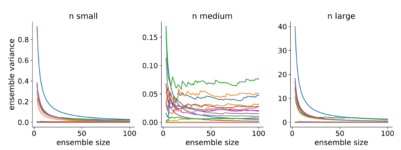
Ensemble variance. The models are stochastic, meaning each time we run them the results will be different. We want to know how much variance there is across multiple runs. We run each model a total of 100 times and measure the variance in the results. We do this separately for each model and each output. Then, for each output, we average the variance across all models. Note that it is not necessary to calculate ensemble variance for each parameter set, but as there are only 16 models, we have the computational resources to measure them all. Figure 10 shows the results. We can see that the ensemble variance has stabilised for each output at an ensemble size of 100 runs.
To calculate ensemble variance for a given model \(j\), we measure the difference between each ensemble run with each other ensemble run using MASE (see Equation 8). Given 100 runs, this makes for a total of 4950 comparisons.
First, the set of comparisons is given as
| \[D^r_j = \bigcup_{a = 1}^{99} \bigcup_{b = a+1}^{100} \max\{V^{rj}_{m}(f^r_a(x), f^r_b(x)),\ \ V^{rj}_{m}(f^r_b(x), f^r_a(x))\}, \] | \[(9)\] |
Next, we calculate the variance of the set of ensemble runs given in Equation 9. This is:
| \[V^r_j = \frac{1}{4949} \sum_a^{4950} \left( D^r_{j_a} - E(d^r_j) \right)^2, \] | \[(10)\] |
Finally, we calculate the average ensemble variance across the 16 models for output \(r\) as
| \[V^r_e = \frac{1}{16} \sum_{j=1}^{16} V^r_j. \] | \[(11)\] |
Results
Three waves of HM were performed, after which HM was unable to reduce the non-implausible space any further, so the procedure was stopped. In the first wave, the non-implausible space was reduced from 16 scenarios to seven. The second wave further reduced the plausible space to four scenarios. Table 2 shows the four models that were found to be plausible and which factors were switched on. These results match those in Ge et al. (2018), who use POM to select plausible models. The common feature of these four models is that succession and leisure are always turned on, whereas the remaining two factors (diversification and industrialisation) are mixed.
| Model ID | Succ. | Leisure | Divers. | Indust. |
|---|---|---|---|---|
| 13 | x | x | x | |
| 14 | x | x | ||
| 15 | x | x | x | x |
| 16 | x | x | x | |
Table 3 shows the ensemble variances (\(V_e\)) and model discrepancies (\(V_m\)) in each wave. There is little stochasticity in the model as shown by the relatively small ensemble variances, whereas there is noticeable discrepancy between the model result and empirical data. Therefore ensemble variance has little effect on the implausibility score of each model, whilst model discrepancy has a strong effect.
| small | medium | large | ||
|---|---|---|---|---|
| wave 1 | \(V_s\) | 0.028 | 0.035 | 0.025 |
| \(V_m\) | 7.568 | 5.335 | 17.539 | |
| wave 2 | \(V_s\) | 0.037 | 0.046 | 0.029 |
| \(V_m\) | 4.493 | 4.115 | 7.182 | |
| wave 3 | \(V_s\) | 0.004 | 0.003 | 0.007 |
| \(V_m\) | 1.805 | 2.229 | 5.551 | |
HM has helped narrow down our list of plausible models from 16 to four. This reduction of the parameter space was achieved quickly (with 1600 model-runs) compared to the number of runs that would be required with alternative calibration methods. The result also matches that found using POM (Ge et al. 2018). However, HM does not provide the probability that these four models can accurately match the empirical data. Instead, each model is considered equally plausible. To gain insight into the probabilities, we use the rejection sampling method of ABC.
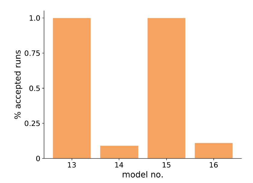
We initially set \(\epsilon\) to be the sum of the uncertainties found in the final wave of HM, as given in Table 3. We ran each of the four models 100 times, resulting in 53 runs of model 13 accepted, and no runs of the remaining three models. Increasing this threshold by \(0.95\), however, resulted in most runs being accepted for models 13 and 15, and less than a quarter of the runs accepted for models 14 and 16 (see Figure 11). If the threshold is any lower, than no runs for 14 or 16 are accepted, but over 90 are accepted for 13 and 15. These results suggest that models 13 and 15 have the best probability of successfully simulating changes in the size of Scottish cattle farms over time. Both of these models include industrialisation (as well as succession and leisure) as part of the farm holder’s decision making. Models 14 and 16, which are less likely to match the empirical data, do not include industrialisation.
Through ABC rejection sampling, we have found the best models that fit the empirical data and have learnt the relative importance of each of the four factors considered. This was achieved through measuring the uncertainties associated with the model and using those uncertainties to help choose appropriate thresholds for the rejection sampling procedure.
Discussion
We used two models to demonstrate the utility of the proposed framework. First, we use the territorial birds model to compare our proposed approach against existing approaches. Thiele et al. (2014) demonstrate a range of calibration methods on the model, including random sampling, simulated annealing and ABC. We showed that by performing HM before ABC, we can obtain equivalent results to using ABC alone using considerably fewer runs of the model, thus saving on computational time. We can also obtain an accurate prior with HM alone, which is useful for cases where performing ABC afterwards is computationally infeasible. This is achieved through identifying the uncertainties of the model.
We also demonstrate that HM provides more information than point-estimation calibration methods, as it provides a region of parameters that perform well whilst also accounting for uncertainties in the model and data. While this required more runs of the model than a point-estimation method, the information gained is valuable.
Second, for the farming example (the RISC model), HM helped to rule out the implausible models. Specifically, models without leisure and succession are not chosen, which is consistent with model selection using POM (Ge et al. 2018). Our approach enhances our understanding of the role of different processes that co-exist in the Scottish dairy farms. We have found that the lack of succession (which explains the increasing number of small farms) and leisure (which explains the existence of non-profitable small farms) are the primary driving forces behind the polarisation of Scottish dairy farms.
In addition to HM, ABC further distinguishes models with industrialisation (employing a professional manager to help expand a farm) as having a higher probability of matching the empirical data than those without. This indicates that although industrialisation may not be the primary driving force of the trend of polarisation, it is likely that it does play a role. This role may explain the increasing number of large farms. Without considering industrialisation, the model fails to capture the growth of large farms. This finding is new, and was not picked up by POM previously, or by HM alone. The reason is that both POM and HM are categorical, so they accept models both with and without industrialisation elements, as they are all plausible. ABC, however, estimates that models with industrialisation have a higher probability of matching the data than those without. This new insight is a direct consequence of combining HM with ABC to calibrate an ABM.
If a point-estimation method of calibration was used on the RISC model, we would only discover a single best fitting model and would have not discovered that multiple models provide a good fit, which has lead to a better understanding of the factors that affect farmers’ decision making. The advantage of using ABC over POM is that we are able to find the probabilities that these factors affect decision making. Furthermore, by using HM before ABC we were able to discover this with significantly fewer runs than would have been required with ABC alone (because the sample space was narrowed to a more accurate region by HM), thereby saving computational time.
Conclusions
Designing and calibrating ABMs is a challenge due to uncertainties around the parameters, model structure and stochasticity of such models. We have illustrated a process of calibrating an ABM’s structure and parameters that quantifies these uncertainties through the combined use of HM and ABC. The code and results used in this paper are all available online at https://github.com/Urban-Analytics/uncertainty.
We show that HM can be used to efficiently reduce parameter space uncertainties; moreover, by quantifying the model uncertainties it is only necessary to test each chosen parameter once. Following this, ABC provides a more detailed exploration of the remaining parameter space, quantifying uncertainties in terms of a probability distribution over non-implausible values.
We demonstrate this process with a toy example (Sugarscape) and two models of real-world processes, which simulate the movement of territorial birds and the changing sizes of cattle farms in Scotland. In the territorial birds model, we demonstrate that our approach is more informative than point-estimation calibration methods, and more efficient than Bayesian calibration methods alone without HM. We show that the number of model-runs required for calibration is approximately halved if HM is used before ABC, compared to using ABC alone. While this is shown with a simple model and simple ABC method, we believe that using HM will be beneficial with more complex models even when more efficient methods of ABC (e.g., sequential Monte Carlo) are used. In the farming model, we show that HM was able to test competing sociological theories and removed all models with a structure that was expected to be implausible based on an alternative POM approach (Ge et al. 2018). We then show that ABC provides insights into the factors that are important in Scottish cattle farmers when deciding to change the size of their farm.
As the number of parameters in a model increases, the resources required to calibrate the model grows to become prohibitive. We have suggested using HM to quickly find a narrow area of the search space, which can then be explored in more detail with a rigorous approach, such as ABC. For a particularly large parameter space or computational demanding model, one could use the non-implausible space found by HM to build a surrogate model. This simpler surrogate may be used in place of the real model to carry out ABC with more feasible resources (Lamperti et al. 2018).
In future work, we will explore our proposed approach further using new results generated with the RISC model. We will create true data generated using the best fitting parameters found in this paper and investigate if our method still finds the correct parameters to be the most likely sets to fit our true data.
If ABMs are to achieve their potential as a go to tool for policymakers and academics, robust calibration and uncertainty quantification handling methods need to be developed. Using the proposed process, calibration of ABMs can be carried out efficiently whilst taking into account all uncertainties associated with the model and the real-world process.
Acknowledgements
This project has received funding from the European Research Council (ERC) under the European Union’s Horizon 2020 research and innovation programme (grant agreement No. 757455) and was supported by The Alan Turing Institute. AH was also supported by grants from UKPRP (MR/S037578/2), Medical Research Council (MC_UU_00022/5) and Scottish Government Chief Scientist Office (SPHSU20). We also gratefully acknowledge the effort made by the reviewers to help improve this manuscript.Notes
Note that in three of the 91 tests, although the plausible range for survival probability contains the true value, if our precision was higher (to 4 d.p. instead of 3 d.p.) these cases would have been rejected↩︎
Appendix: Notation
See Table 4 for a list of mathematical notation used in the paper.
| Term | Meaning |
|---|---|
| \(R\) | total observations/outputs |
| \(z^r\) | the \(r^{\text{th}}\) observation |
| \(f^r(x)\) | the \(r^{\text{th}}\) model output |
| \(f^{rj}(x)\) | the \(r^{\text{th}}\) of the \(j^{\text{th}}\) (RISC example) |
| \(d(z^r, f^r(x)\) | error measure between the \(r^{\text{th}}\) model output and observation |
| \(N\) | total parameters sampled |
| \(x_n\) | the \(n^{\text{th}}\) parameter set |
| \(v_o^r\) | observation variance of the \(r^{\text{th}}\) observation |
| \(v_s^r\) | ensemble variance of the \(r^{\text{th}}\) output |
| \(v_m^r\) | model discrepancy of the \(r^{\text{th}}\) output |
| \(I^r(c)\) | implausibility measure of the \(r^{\text{th}}\) output |
| \(c\) | implausibility threshold |
| \(S\) | total runs in an ensemble |
References
ABDULKAREEM, S. A., Mustafa, Y. T., Augustijn, E.-W., & Filatova, T. (2019). Bayesian networks for spatial learning: A workflow on using limited survey data for intelligent learning in spatial agent-based models. GeoInformatica, 23(2), 243–268. [doi:10.1007/s10707-019-00347-0]
ANDRIANAKIS, I., Vernon, I. R., McCreesh, N., McKinley, T. J., Oakley, J. E., Nsubuga, R. N., Goldstein, M., & White, R. G. (2015). Bayesian history matching of complex infectious disease models using emulation: A tutorial and a case study on HIV in Uganda. PLoS Computational Biology, 11(1), e1003968. [doi:10.1371/journal.pcbi.1003968]
ARENDT, P. D., Apley, D. W., & Chen, W. (2012). Quantification of model uncertainty: Calibration, model discrepancy, and identifiability. Journal of Mechanical Design, 134, 100908. [doi:10.1115/1.4007390]
BEAUMONT, M. A., Zhang, W., & Balding, D. J. (2002). Approximate Bayesian computation in population genetics. Genetics, 162(4), 2025–2035. [doi:10.1093/genetics/162.4.2025]
COOKE, R. M., & Goossens, L. L. H. J. (2008). TU Delft expert judgment data base. Reliability Engineering & System Safety, 93(5), 657–674. [doi:10.1016/j.ress.2007.03.005]
CRAIG, P. S., Goldstein, M., Seheult, A. H., & Smith, J. A. (1997). 'Pressure matching for hydrocarbon reservoirs: A case study in the use of Bayes linear strategies for large computer experiments.' In C. Gatsonis, J. S. Hodges, R. E. Kass, R. McCulloch, P. Rossi, & N. D. Singpurwalla (Eds.), Case Studies in Bayesian Statistics (Vol. 3, pp. 37–93). Berlin Heidelberg: Springer. [doi:10.1007/978-1-4612-2290-3_2]
CROLS, T., & Malleson, N. (2019). Quantifying the ambient population using hourly population footfall data and an agent-based model of daily mobility. GeoInformatica, 23(2), 201–220. [doi:10.1007/s10707-019-00346-1]
CROOKS, A., Castle, C., & Batty, M. (2008). Key challenges in agent-Based modelling for geo-Spatial simulation. Computers, Environment and Urban Systems, 32(6), 417–430. [doi:10.1016/j.compenvurbsys.2008.09.004]
CSILLÉRY, K., Blum, M. G. B., Gaggiotti, O. E., & François, O. (2010). Approximate Bayesian Computation (ABC) in practice. Trends in Ecology & Evolution, 25(7), 410–418.
DALY, A. C., Cooper, J., Gavaghan, D. J., & Holmes, C. (2017). Comparing two sequential Monte Carlo samplers for exact and approximate Bayesian inference on biological models. Journal of the Royal Society Interface, 14(134), 20170340. [doi:10.1098/rsif.2017.0340]
DEL Moral, P., Doucet, A., & Jasra, A. (2012). An adaptive sequential Monte Carlo method for Approximate Bayesian Computation. Statistics and Computing, 22(5), 1009–1020. [doi:10.1007/s11222-011-9271-y]
EPSTEIN, J. M., & Axtell, R. (1996). Growing Artificial Societies: Social Science from the Bottom Up. Washington, DC: Brookings Institution Press.
FEARNHEAD, P., & Künsch, H. R. (2018). Particle filters and data assimilation. Annual Review of Statistics and Its Application, 5(1), 421–449. [doi:10.1146/annurev-statistics-031017-100232]
FILATOVA, T., Verburg, P. H., Parker, D. C., & Stannard, C. A. (2013). Spatial agent-Based models for socio-Ecological systems: Challenges and prospects. Environmental Modelling & Software, 45, 1–7. [doi:10.1016/j.envsoft.2013.03.017]
GE, J., Polhill, J. G., Matthews, K. B., Miller, D. G., & Spencer, M. (2018). Not one Brexit: How local context and social processes influence policy analysis. PloS ONE, 13(12), e0208451. [doi:10.1371/journal.pone.0208451]
GRAZZINI, J., Richiardi, M. G., & Tsionas, M. (2017). Bayesian estimation of agent-Based models. Journal of Economic Dynamics and Control, 77, 26–47. [doi:10.1016/j.jedc.2017.01.014]
GRIMM, V., Revilla, E., Berger, U., Jeltsch, F., Mooij, W. M., Railsback, S. F., Thulke, H.-H., Weiner, J., Wiegand, T., & DeAngelis, D. L. (2005). Pattern-Oriented modeling of agent-Based complex systems: Lessons from ecology. Science, 310(5750), 987–991. [doi:10.1126/science.1116681]
HASSAN, S., Arroyo, J., Galán, J. M., Antunes, L., & Pavón, J. (2013). Asking the oracle: Introducing forecasting principles into agent-based modelling. Journal of Artificial Societies and Social Simulation, 16(3), 13: https://www.jasss.org/16/3/13.html. [doi:10.18564/jasss.2241]
HEPPENSTALL, A., Crooks, A., Malleson, N., Manley, E., Ge, J., & Batty, M. (2020). Future developments in geographical agent-Based models: Challenges and opportunities. Geographical Analysis, 53(1), 76–91. [doi:10.1111/gean.12267]
HEPPENSTALL, A. J., Evans, A. J., & Birkin, M. H. (2007). Genetic algorithm optimisation of an agent-based model for simulating a retail market. Environment and Planning B: Planning and Design, 34(6), 1051–1070. [doi:10.1068/b32068]
HUTH, A., & Wissel, C. (1994). The simulation of fish schools in comparison with experimental data. Ecological Modelling, 75, 135–146. [doi:10.1016/0304-3800(94)90013-2]
KAZIL, J., Masad, D., & Crooks, A. (2020). 'Utilizing python for agent-Based modeling: The Mesa framework.' In R. Thomson, H. Bisgin, C. Dancy, A. Hyder, & M. Hussain (Eds.), Social, Cultural, and Behavioral Modeling (pp. 308–317). Cham: Springer International Publishing. [doi:10.1007/978-3-030-61255-9_30]
KENNEDY, M. C., & O’Hagan, A. (2001). Bayesian calibration of computer models. Journal of the Royal Statistical Society: Series B (Statistical Methodology), 63(3), 425–464. [doi:10.1111/1467-9868.00294]
LAMPERTI, F., Roventini, A., & Sani, A. (2018). Agent-based model calibration using machine learning surrogates. Journal of Economic Dynamics and Control, 90, 366–389. [doi:10.1016/j.jedc.2018.03.011]
LEI, C. L., Ghosh, S., Whittaker, D. G., Aboelkassem, Y., Beattie, K. A., Cantwell, C. D., Delhaas, T., Houston, C., Novaes, G. M., Panfilov, A. V., Pathmanathan, P., Riabiz, M., dos Santos, R. W., Walmsley, J., Worden, K., Mirams, G. R., & Wilkinson, R. D. (2020). Considering discrepancy when calibrating a mechanistic electrophysiology model. Philosophical Transactions of the Royal Society A: Mathematical, Physical and Engineering Sciences, 378(2173), 20190349. [doi:10.1098/rsta.2019.0349]
LENORMAND, M., Jabot, F., & Deffuant, G. (2013). Adaptive approximate Bayesian computation for complex models. Computational Statistics, 28(6), 2777–2796. [doi:10.1007/s00180-013-0428-3]
LI, T., Cheng, Z., & Zhang, L. (2017). Developing a novel parameter estimation method for agent-Based model in immune system simulation under the framework of history matching: A case study on Influenza A virus infection. International Journal of Molecular Sciences, 18(12), 2592. [doi:10.3390/ijms18122592]
MANSON, S., An, L., Clarke, K. C., Heppenstall, A., Koch, J., Krzyzanowski, B., Morgan, F., O’Sullivan, D., Runck, B. C., Shook, E., & Tesfatsion, L. (2020). Methodological issues of spatial agent-based models. Journal of Artificial Societies and Social Simulation, 23(1), 3: https://www.jasss.org/23/1/3.html. [doi:10.18564/jasss.4174]
MARIN, J.-M., Pudlo, P., Robert, C. P., & Ryder, R. J. (2012). Approximate Bayesian Computational methods. Statistics and Computing, 22(6), 1167–1180. [doi:10.1007/s11222-011-9288-2]
MOYA, I., Chica, M., & Cordón, O. (2021). Evolutionary multiobjective optimization for automatic agent-Based model calibration: A comparative study. IEEE Access, 9, 55284–55299. [doi:10.1109/access.2021.3070071]
NERI, F. (2018). Combining machine learning and agent-based modeling for gold price prediction. Italian Workshop on Artificial Life and Evolutionary Computation. [doi:10.1007/978-3-030-21733-4_7]
O’HAGAN, A., Buck, C. E., & Daneshkhah, A. (2006). Uncertain Judgements: Eliciting Experts’ Probabilities. Hoboken, NJ: John Wiley & Sons.
PAPADELIS, S., & Flamos, A. (2019). 'An application of calibration and uncertainty quantification techniques for agent-Based models.' In H. Doukas, A. Flamos, & J. Lieu (Eds.), Understanding Risks and Uncertainties in Energy and Climate Policy: Multidisciplinary Methods and Tools for a Low Carbon Society (pp. 79–95). Cham: Springer International Publishing. [doi:10.1007/978-3-030-03152-7_3]
PIETZSCH, B., Fiedler, S., Mertens, K. G., Richter, M., Scherer, C., Widyastuti, K., Wimmler, M.-C., Zakharova, L., & Berger, U. (2020). Metamodels for evaluating, calibrating and applying agent-Based models: A review. Journal of Artificial Societies and Social Simulation, 23(2), 9: https://www.jasss.org/23/2/9.html. [doi:10.18564/jasss.4274]
POLHILL, J. G., Ge, J., Hare, M. P., Matthews, K. B., Gimona, A., Salt, D., & Yeluripati, J. (2019). Crossing the chasm: A “tube-map” for agent-based social simulation of policy scenarios in spatially-distributed systems. GeoInformatica, 23(2), 169–199. [doi:10.1007/s10707-018-00340-z]
PUKELSHEIM, F. (1994). The three sigma rule. The American Statistician, 48(2), 88–91. [doi:10.1080/00031305.1994.10476030]
PURSHOUSE, R. C., Ally, A. K., Brennan, A., Moyo, D., & Norman, P. (2014). Evolutionary parameter estimation for a theory of planned behaviour microsimulation of alcohol consumption dynamics in an English birth cohort 2003 to 2010. Proceedings of the 2014 Annual Conference on Genetic and Evolutionary Computation, New York, NY, USA. [doi:10.1145/2576768.2598239]
RAILSBACK, S. F., & Grimm, V. (2019). Agent-Based and individual-Based modeling: A practical introduction. Princeton University Press.
ROUCHIER, J., Bousquet, F., Requier-Desjardins, M., & Antona, M. (2001). A multi-Agent model for describing transhumance in North Cameroon: Comparison of different rationality to develop a routine. Journal of Economic Dynamics and Control, 25(3), 527–559. [doi:10.1016/s0165-1889(00)00035-x]
SMITH, R. C. (2013). Uncertainty Quantification: Theory, Implementation, and Applications. Society for Industrial; Applied Mathematics.
STAVRAKAS, V., Papadelis, S., & Flamos, A. (2019). An agent-Based model to simulate technology adoption quantifying behavioural uncertainty of consumers. Applied Energy, 255(1), 113795. [doi:10.1016/j.apenergy.2019.113795]
STRONG, M., Oakley, J. E., & Chilcott, J. (2012). Managing structural uncertainty in health economic decision models: A discrepancy approach. Journal of the Royal Statistical Society: Series C (Applied Statistics), 61(1), 25–45. [doi:10.1111/j.1467-9876.2011.01014.x]
STURLEY, C., Newing, A., & Heppenstall, A. (2018). Evaluating the potential of agent-based modelling to capture consumer grocery retail store choice behaviours. The International Review of Retail, Distribution and Consumer Research, 28(1), 27–46. [doi:10.1080/09593969.2017.1397046]
SUNNÅKER, M., Busetto, A. G., Numminen, E., Corander, J., Foll, M., & Dessimoz, C. (2013). Approximate bayesian computation. PLoS Computational Biology, 9(1), e1002803.
TEN Broeke, G., van Voorn, G., & Ligtenberg, A. (2016). Which sensitivity analysis method should I use for my agent-Based model? Journal of Artificial Societies and Social Simulation, 19(1), 5: https://www.jasss.org/19/1/5.html. [doi:10.18564/jasss.2857]
THIELE, J. C., Kurth, W., & Grimm, V. (2014). Facilitating parameter estimation and sensitivity analysis of agent-Based models: A cookbook using NetLogo and ’R’. Journal of Artificial Societies and Social Simulation, 17(3), 11: https://www.jasss.org/17/3/11.html. [doi:10.18564/jasss.2503]
TONI, T., Welch, D., Strelkowa, N., Ipsen, A., & Stumpf, M. P. (2009). Approximate Bayesian Computation scheme for parameter inference and model selection in dynamical systems. Journal of the Royal Society Interface, 6(31), 187–202. [doi:10.1098/rsif.2008.0172]
TURNER, B. M., & Van Zandt, T. (2012). A tutorial on Approximate Bayesian Computation. Journal of Mathematical Psychology, 56(2), 69–85. [doi:10.1016/j.jmp.2012.02.005]
VAN der Vaart, E., Beaumont, M. A., Johnston, A. S. A., & Sibly, R. M. (2015). Calibration and evaluation of individual-Based models using Approximate Bayesian Computation. Ecological Modelling, 312, 182–190. [doi:10.1016/j.ecolmodel.2015.05.020]
VERNON, I., Goldstein, M., Bower, R. G., & others. (2010). Galaxy formation: A bayesian uncertainty analysis. Bayesian Analysis, 5(4), 619–669. [doi:10.1214/10-ba524]
WALDROP, M. M. (2018). Free agents. Science, 360(6385), 144–147. [doi:10.1126/science.360.6385.144]
WEISS, C. R. (1999). Farm growth and survival: Econometric evidence for individual farms in Upper Austria. American Journal of Agricultural Economics, 81(1), 103–116. [doi:10.2307/1244454]
WINDRUM, P., Fagiolo, G., & Moneta, A. (2007). Empirical validation of agent-Based models: Alternatives and prospects. Journal of Artificial Societies and Social Simulation, 10(2), 8: https://www.jasss.org/10/2/8.html.
ZHANG, H., Vorobeychik, Y., Letchford, J., & Lakkaraju, K. (2016). Data-driven agent-based modeling, with application to rooftop solar adoption. Autonomous Agents and Multi-Agent Systems, 30(6), 1023–1049. [doi:10.1007/s10458-016-9326-8]
ZOELLNER, C., Jennings, R., Wiedmann, M., & Ivanek, R. (2019). EnABLe: An agent-Based model to understand Listeria dynamics in food processing facilities. Scientific Reports, 9(1), 1–14. [doi:10.1038/s41598-018-36654-z]