Abstract

This paper presents a set of guidelines, imported from the field of forecasting, that can help social simulation and, more specifically, agent-based modelling practitioners to improve the predictive performance and the robustness of their models. The presentation starts with a discussion on the current debate on prediction in social processes, followed by an overview of the recent experience and lessons learnt from the field of forecasting. This is the basis to define standard practices when developing agent-based models under the perspective of forecasting experimentation. In this context, the guidelines are structured in six categories that correspond to key issues that should be taken into account when building a predictor agent-based model: the modelling process, the data adequacy, the space of solutions, the expert involvement, the validation, and the dissemination and replication. The application of these guidelines is illustrated with an existing agent-based model. We conclude by tackling some intrinsic difficulties that agent-based modelling often faces when dealing with prediction models.

Keywords:

Forecasting, Guidelines, Prediction, Agent-Based Modelling, Modelling Process, Social Simulation

Introduction

1.1

The technique of Agent-Based Modelling (ABM) has become widely used for research in Social Sciences (Gilbert & Troitzsch, 1999), especially for understanding social phenomena or to validate social theories. Given its ability to show the evolution of complex systems, one question arises: can ABM support forecasting? This issue has risen lively discussions, until a point where many prefer to avoid dealing with this hornets' nest.

1.2

In 2009, Scott Moss asked in the SIMSOC¹ list if anyone could point out a correct model-based forecast of the impact of any social policy² (that is, a forecast prior to the implementation of the policy). After long discussions and once misunderstandings were sorted out, no one could. This led consequently to question the point of agent-based simulation, since it has no forecasting capability, starting another heated debate³.

1.3

Current agent-based models do not reach the prediction capabilities that stake-holders would desire, and this fact feeds the continuous need of ABM to 'defend' and justify its existence. In this context, the role that prediction should play in ABM can be very different depending on the researcher. Many researchers, such as Joshua Epstein (Epstein, 2008), place prediction as a secondary objective, arguing that there are many other possible reasons to build models. In fact, he lists 16 of them, including explanation, guiding data collection, raising new questions or suggesting analogies. He stresses his point stating that 'Explanation does not imply Prediction', the same way as Tectonics explains earthquakes but cannot predict them.

1.4

An interesting reply to these arguments, by Thompson & Derr (2009), considers that 'good explanations predict', as explanatory models must appropriately predict real behaviours if they expect to be considered valid. This is very related to the issue of when a model is considered 'correct' or 'validated' (Galán et al., 2009). Troitzsch (2009) joins the debate with an important clarification on the meanings of prediction, arguing that Epstein and Thompson discuss over different concepts. He defines three levels of prediction:

1. Prediction of the kind of behaviour of a system, under arbitrary parameter combinations and initial conditions: ''Earthquakes occur because X and Y.''
2. Prediction of the kind of behaviour of a system in the near future: ''Region R is likely to suffer earthquakes in the following years because X and Y.''
3. Prediction of the state a system will reach in the near future: ''Region R will suffer an earthquake of power P in expected day D with confidence C.''

1.5

Troitzsch argues that explanation does not have to imply the third level prediction (Epstein's statement refined), but that good explanations usually imply first and even second level predictions (Thompson and Derr's point refined). In fact, Heath et al. (2009) propose a similar classification, which can be redefined as follows: Generators are models whose aim is first level prediction (theoretical understanding); Mediators are those whose aim is second level prediction (insight of behaviour); and Predictors are models seeking third level prediction (estimation). From this approach, Moss's debate in SIMSOC can be seen as the difficulty to find a Predictor model that has been already applied for third level prediction with success.

1.6

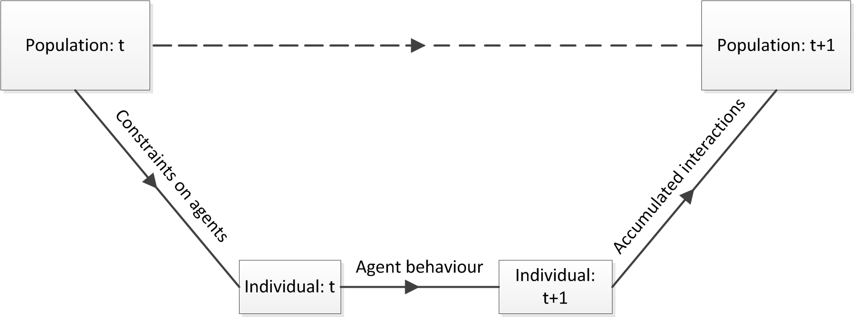
Many of the agent-based models in the literature have an explanatory vocation. The sheer choice of using an agent-based model to represent a target system implicitly indicates a purpose to model the underlying generative mechanisms that are governing the dynamics. Although this can seem puzzling, this fact can hinder the options to make good predictions. The theoretical framework often used in agent-based social models is based on the Coleman's boat or Coleman (1990) bathtub (see Fig. 1). Understanding (or predicting) the evolution of an aggregated variable under this paradigm requires to establish a macro-micro linkage and to explicitly model the individual micro-behaviour, affected by the macrovariables and affecting them as well. Using the ABM approach obliges to break the system up in entities and interactions, to create a detailed simulation model as inference tool and finally to aggregate the interaction of the entities in order to understand the dynamics of the system. In many cases, this set of tasks implies more work than when non-explicative prediction is the only goal. In this latter case, just using correlated data, not necessarily causal, may outperform an agent-based model. The effort involved in designing an agent-based model is only justified if the modeller is interested in 'how' the phenomenon occurs and not just in 'what' is going to happen. Moreover, in some complex systems that present chaotic regimes, arbitrarily small variations in the initial conditions can lead to very different trajectories. This implies that in those cases it is demonstrably impossible to create models of the third level of prediction proposed by Troitzsch. Many social systems are modelled by features such as stochastic behavior, non-ergodicity or structural changes over time. Given current models, is it possible to reach the third level of prediction?

Figure 1: Adapted from Coleman's bathtub (Coleman, 1990)

1.7

Forecasting is a field that focuses on the study of prediction, especially the aforementioned third level. It has been applied in many contexts for decades, and this experience has driven to the establishment of a set of principles that could be reviewed for ABM, should this be applied as a tool for making predictions. Many of these principles can simply be viewed as good science principles. However, they are usually neglected when making predictions. A paradigmatic example is the 2007 report issued by the Intergovernmental Panel on Climate Change's working group (IPCC), which predicted dramatic increases in average world temperatures over the next 92 years. However, the audit of the report carried out by forecasting experts (Green & Armstrong, 2007) revealed that the forecasting procedures described in the IPCC violated 72 out of 140 forecasting principles, many of them critical.

1.8

The forecasting principles can be seen as an extension of the scientific method. Consequently, they are useful for building any simulation model and not only when forecasting is one of the goals of the simulation. Even if building valid models of social systems is an arduous challenge, that should not prevent social scientists from aiming to strengthen their models with procedures that increase their scientific validity. This paper explores how such forecasting principles can be applied in ABM.

1.9

The next section presents some basics of the forecasting theory, while section 3 adapts some of its core ideas to ABM. Then, section 4 applies well-established forecasting principles to provide a set of initial guidelines to strengthen the development of Predictor agent-based models. Section 5 illustrates the application of these guidelines with an agent-based model of domestic water management, which integrates different submodels with detailed geographical environments. Finally, section 6 exposes some challenges and concluding remarks.

Forecasting: The field in a nutshell

2.1

Forecasting is the process of making statements about future events. Forecasts are needed when there is uncertainty about a future outcome. In such cases, formal forecasting procedures can be useful to reduce the uncertainty in order to make better decisions, especially if poor forecasts can lead to disastrous decisions. Even though some people distinguish between prediction and forecast, we will not distinguish between both terms. However, we prefer the term forecast because the scientific field dealing with this matter is known as Forecasting.

2.2

Forecasting methods are usually classified as either subjective or objective. Subjective methods are those based on judgements and opinions. The most popular subjective method is the Delphi method (Dalkey & Helmer, 1963) which asks for a prediction to a panel of experts for several rounds, expecting that the prediction converges towards the 'correct' value. Objective methods refer to quantitative (statistical) methods, which can be divided into extrapolative and regression methods. The first group considers that the forecast is function only of time and past values of the variable of interest and not of other variables. It includes techniques such as autoregressive models (Box & Jenkins, 1970) or exponential smoothing (Gardner, 2006). The second group tries to estimate the effects of causal variables and includes econometric models (Mills, 2006) amongst others. See Armstrong (2001) for a taxonomy of forecasting methods.

2.3

In the 80's the Forecasting discipline took a major boost with the foundation of the International Institute of Forecasters (IIF), the celebration of the first International Symposium on Forecasting in 1981, and the foundation of the two major forecasting journals (Journal of Forecasting and International Journal of Forecasting). IIF is an organisation dedicated to developing the generation, distribution, and use of knowledge on forecasting. The aim of the institute is to foster progress in forecasting. In order to do so it encourages empirical comparisons of reasonable forecasting approaches using the method of multiple working hypotheses (Chamberlin, 1965).

2.4

This approach was developed by T. C. Chamberlin in the 19th-century and nowadays it is considered an important landmark as philosophical contribution to science (Chamberlin, 1965). According to this approach, the proposed forecasting method should be compared against other leading methods. The conditions under which the experiments are carried out should be well-specified, for example, the characteristics of the data set. Evaluation criteria that make possible to determine what constitutes a better performance should be clearly stated and the results of all the methods according to these criteria should be reported. These ideas are shown in depth in Armstrong & Fildes (2006), an article in the silver anniversary issue of the International Journal of Forecasting that reviews the achievements in the discipline in the last 25 years.

2.5

Unfortunately, according to the review in Armstrong (2006), the method of multiple working hypotheses is seldom used in fields such as social and management sciences. The article also summarises evidence-based findings in forecasting in the period between 1981 and 2006 as a list of basic generalisations that should guide forecasting. This list is the following:

• Be conservative when uncertain: It means that methods that follow conservative assumptions in the face of uncertainty usually work better than those that follow more radical assumptions.
• Spread risk: In forecasting, combining the results of different methods, and the application of the divide and conquer principle (such as time series decomposition) usually obtain better performance than relying on just the single best method.
• Use realistic representations of the situation: Representing situations in a realistic manner is expected to be helpful to improve forecast accuracy. However, realism involves adding some complexity, which has to be carefully done as the law of parsimony (or Occam's razor principle) advises the use of simple methods unless empirical evidence calls for a more complex approach.
• Use lots of information: Methods that use more information (e.g., combining, prediction markets) are superior to those that rely on a single source (e.g., extrapolative methods).
• Use prior knowledge: Methods based on prior knowledge about the situation and relationships (e.g., econometric methods) are superior to those that rely only on the data (e.g., extrapolative methods and data mining).
• Use structured methods: Structured methods consist of detailed steps that can be described and replicated and are usually more accurate than unstructured methods.

2.6

These ideas are further developed in the book Principles of Forecasting (Armstrong, 2001), which proposes guidelines to improve the effectiveness of a forecasting process. The application of a selection of these guidelines to ABM will be illustrated in section 4.

Developing a simulation model following the procedure used in forecasting

3.1

In the forecasting literature, simulation models are not usually regarded as forecasting tools. For instance, they do not appear in the taxonomy of forecasting methods in Armstrong (2001). The reason is that simulation models, ABM included, are frequently used for other purposes, different from forecasting. It can be argued that ABM offers an insight on complex aspects such as the evolution of different but related outputs, the prediction of a distribution of values, the volatility of a phenomenon, or the occurrence of turning points and structural breaks, to cite a few. However, this kind of aspects have been also covered by the forecasting literature on the topics of multiple time series (Lütkepohl, 2007), symbolic time series (Arroyo et al., 2010), volatility models (Engle, 1982; Bollerslev, 1986) and structural breaks (Canova & Ciccarelli, 2004; Pesaran et al., 2006), respectively. In most cases, it would be a futile effort to compare the accuracy of dedicated forecasting tools with an agent-based model. As stated before, the strength of ABM lies on its explanatory power, which usually does not imply accurate forecasts.

3.2

In fact, the impossibility of using ABM to forecast certain phenomena is widely acknowledged in fields such as artificial stock markets. In social sciences, Moss (2008) claims that ABM cannot be used reliably to forecast the consequences of social processes because they produce unpredictable episodes of volatility in macro-level time series. However, the ABM community frequently shares concerns on how to use ABM as a forecasting tool, as shown in the discussion in section 1. From our point of view, it is a difficult challenge to attempt to forecast the macro-behaviour of a complex system through a model that should also reproduce its micro-behaviour. Therefore, if forecasting is the aim, it is frequently more appropriate to focus on macro-behaviours (although in some cases, the aim might be to forecast local effects).

3.3

However, we would not go as far as saying that ABM cannot be used as a forecasting tool in any case. We would rather focus on what can be done to perform forecasts with an agent-based model. Even if the attempt proves to be unsuccessful or the goal of the model is not forecasting, ABM can benefit from the application of the procedure used to set up a forecasting experiment, because it is guided by the good science that implies the method of multiple working hypotheses and the aforementioned generalisations.

3.4

From now on, by the term forecast we refer to the prediction of the value of a quantitative variable based on known past values of that variable or other related variables. As a result, most of the ideas exposed below are related with quantitative forecasting and third level prediction, as defined in section 1. These ideas are useful to build Predictor agent-based models where the use of data is more prominent. However, some can be directly used or adapted accordingly to other kinds of agent-based models, as it is shown later on.

3.5

The following subsections review some key concepts of the procedure used in forecasting. We have not intended to offer an exhaustive guide, but a quick introduction to the topic. For more details, interested readers can check relevant works such as Makridakis et al. (1998) or Chatfield (2001).

Splitting the data set

3.6

In a forecasting situation, analysts have data available up to time N, fit their models up to time N, and then make forecasts about the future using the estimated model. This approach requires waiting for future data to assess the accuracy of the forecasts. However, it is often advisable to use the available data to avoid over-fitting and to evaluate the forecasting ability of the model. In order to do so, data can be split in two or three sets.

3.7

The first set is the estimation (or training) set, which is used to adjust the model. The second set is the validation set, which is used to check whether the model that has been adjusted using the training set is accurate or not. The validation set avoids over-fitting, which is the phenomenon where the model describes noise instead of the underlying relationships of interest, and helps to choose a more parsimonious model that also works well in the hold-out data. If the adjusted model is a good representation of the 'true' model, then its forecast accuracy should be high and similar in both data sets.

3.8

However, the statements about the predictive power of the model drawn from the validation set would be biased, since the validation set is used to select the final model. Thus, if the aim is to make a statement about the actual predictive power of the model, we should look into a third data set, the test set. However, the model must not be tuned any further with the information drawn from this third set.

3.9

In ABM, guiding model construction and selection using the aforementioned partitions of the data is useful to avoid over-fitting and to select better models. However, it might occur that using a more parsimonious model does not improve the out-of-sample accuracy. Reasons could include that the model is not adequate or that during the out-of-sample period some structural changes occur that prevent the in-sample adjusted model from forecasting accurately.

Ex-ante and ex-post forecasts

3.10

It is important to distinguish between ex-post and ex-ante accuracy. Ex-post is a Latin term that means 'after the event', while ex-ante means 'before the event'. An ex-ante forecast only uses information available by the time of the actual forecast, while an ex-post forecast takes also into account information of input variables after the time at which the actual forecast is prepared.

3.11

As ex-post forecasts also consider future information, they are expected to be more accurate than ex-ante forecasts, which are genuine predictions of the future (unknown by definition). However, measuring the accuracy of both ex-ante and ex-post forecasts is useful to find out what actually causes forecast errors: bad forecasting model or bad forecast of the variables used by the model. In a simulation model that integrates several subsystems, the use of ex-post forecast is useful to diagnose the subsystems that do not behave as expected.

Measuring forecast accuracy

3.12

The criterium to measure the adequacy of a forecast should ideally reflect the impact of the error into the decision that is going to be taken. Unfortunately, it is usually too complex to establish this kind of criteria. As a result, the criterium is usually the forecast error of the variable of interest, which should be quantitative in order to make measurements possible.

3.13

The forecast error in time t (e_t) is the difference between the forecasted value  and the actual value x_t in time t, i.e.  e_t = - x_t. There are many different ways to aggregate the error in t along time. Each resulting error measure has different properties. In Hyndman & Koehler (2006) there is an interesting review of accuracy measures. The most popular ones are the following:

Root Mean Square Error (RMSE) =

Mean Absolute Error (MAE) = mean(|et|)

Mean Absolute Percentage Error (MAPE) = mean(|et100/xt|)

The RMSE is a measure with interesting statistical properties because the MSE is the second moment (about the origin) of the error, and thus incorporates both the variance of the estimator and its bias. The MAE is a very easily interpretable error measure, while the MAPE is a measure based on percentage errors. Thus, MAPE is scale independent and has a nice interpretation. However, percentage-based error measures require that the domain of the variable of interest has a meaningful zero (e.g., they are not useful to measure errors in time series represented in the Celsius scale).

3.14

The accuracy of the forecasts can be considered as one of the guiding criteria for model construction and it could be the most important to assess the forecasting performance of the model. It is important to take into account that error measures such as the ones cited above require only one time series of forecasts, while in ABM we can obtain different time series of forecasts with each model run. Thus, to assess the accuracy of an agent-based model it is recommended to average a sufficient number of forecasted time series obtained from different model runs.

Comparing against the benchmarks

3.15

The multiple working hypotheses approach serves well to compare the forecasts of a model along those obtained by other methods or models. To do this successfully, three requirements must be met:

1. Compare on the basis of ex-ante performance.
2. Compare forecasts with those from leading simulation models or reasonable forecasting approaches.
3. Use an adequate sample of forecasts.

3.16

Regarding the second point, the simplest time series forecasting method is the naive method, which assumes that the next value of a time series will be equal to the last value, i.e., that no change will occur. If one does not have information about the series, the most sensible thing to say about the future is that everything will remain the same. Despite its simplicity, the naive method provides relatively accurate forecasts in many cases. Thus, it is a reasonable benchmark method. Simple exponential smoothing methods (Gardner, 2006) are other non-sophisticated time series forecasting methods that can be used as benchmarks. Obviously, if there are simulation models or forecasting methods that are known to provide reliable forecasts, they should be included in the comparison.

3.17

It can be discouraging to obtain poor forecasting performance with a simulation model. This may be the case when a comparison against an effective forecasting method is made. If the prediction power is the ultimate goal of the simulation model, then the model should be ruled out. However, simulation models are usually built to explain the dynamics of the studied phenomenon. If this is the case, the explanatory power of the model has to be evaluated.

Guidelines for forecasting with ABM

4.1

The reference book Principles of Forecasting (Armstrong, 2001) summarises the forecasting practice along the years and translates the findings into 139 principles. These principles should guide a forecasting process to make it more effective. In this work, we have filtered, aggregated and worked on these forecasting principles aiming to formulate a set of guidelines to build agent-based models for forecasting. These guidelines are illustrated with multiple references from the ABM literature.

4.2

Note that not all the guidelines are necessarily needed in the same model, nor do we believe that none of them has already been applied in the field. Being the ABM field rather interdisciplinary, these guidelines will sound more familiar to the quantitative-oriented disciplines, used to focus on prediction as the main scientific aim. Thus, one may be tempted to believe that these will be most useful to social scientists rather than to traditional engineers. However, many quantitative data-driven engineer-like agent-based models might be enriched after a thorough review of their models under the light of these guidelines, as it is shown in section 5 with a case study.

4.3

Additionally, we have grouped the selected principles into six categories that represent key issues that should be taken into account when building a predictor agent-based model: modelling process, use of data, space of solutions, stake-holders, validation, and replication. These should serve as guidelines for developing agent-based model for forecasting⁴. However, many of these guidelines might also be useful for other agent-based models whose aim is not accurate prediction. In order to clarify in which cases the guidelines are applicable (i.e. capable of being adopted), we have classified them in Table 1. For the sake of clarity, two general categories of ABM were used in the table: data-driven ABMs (whose main aim is prediction), and abstract theoretical models (that seek understanding).

Table 1: Classification of the guidelines according to their application in Theoretical agent-based models and Data-driven agent-based models

Guideline Code	Guideline	Theoretical ABM	Data-driven ABM
		Aim: Understanding	Aim: Prediction
MP1	Decompose the problem into parts
MP2	Structure problems that involve causal chains
MP3	Consider whether the events or series can be forecasted
MP4	Use theory to guide the search for information on explanatory variables
DA1	Use diverse sources of data
DA2	Select simple methods unless empirical evidence calls for a more complex approach & The method should provide a realistic representation of the situation
SS1	Identify possible outcomes prior to making forecasts
SS2	Adjust for events expected in the future
SS3	Design test situations to match the forecasting problem
EI1	Ask unbiased experts to rate potential methods
EI2	Test the client's understanding of the methods & Obtain decision makers' agreement on methods
EI3	Establish a formal review process to ensure that forecasts are used properly
V1	Specify criteria for evaluating methods prior to analysing data
V2	Use objective tests of assumptions
V3	Establish a formal review process for forecasting methods
A1	Assess acceptability and understandability of methods to users
A2	Describe potential biases of forecasters
A3	Replicate forecast evaluations to assess their reliability
A4	Use extensions of evaluations to better generalise about what methods are best for what situations
A5	Compare track records of various forecasting methods

=> Very frequently applicable
=> Sometimes applicable
=> Very rarely applicable

Modelling Process

•

MP1. Decompose the problem into parts (g.2.3). Do a bottom-up approach and then combine results. This synthetic approach is inherent to ABM. This decomposition is risky, as it might not be unique, and the synthesis might be a harder problem than the target problem itself. However, the idea of approaching a problem with a computational stance necessarily implies some decomposition and synthesis.

•

MP2. Structure problems that involve causal chains (g.2.6). Sometimes it is possible to use the results of some models as inputs to other models, and this allows for better accuracy than simulating everything simultaneously. Some agent-based models follow this guideline structuring the models in different coupled layers, each level implementing a submodel, which is used as an input for the others. In those cases, we can find the coupling of agent-based models with statistical or equation-based models (Galán et al., 2009; Athanasiadis et al., 2005). An interesting example is Bithell & Brasington (2009) in which an agent-based model is combined with an individual-based model and a spatial hydrological model.

•

MP3. Consider whether the events or series can be forecasted (g.1.4). There are multiple contexts in which the (level 3) accurate prediction is simply not possible. If sample forecasts cannot improve the naive benchmark, this might be the case (check section 3.4 for details). Typically, forecasting in stock markets is usually not possible. As a result, stock market simulations focus on reproducing stylised facts, i.e., empirical properties that are so consistent that they are accepted as valid⁵ (Lux & Marchesi, 1999).

•

MP4. Use theory to guide the search for information on explanatory variables (g.3.1). Even in utmost complex problems, there are some 'truths' and 'facts' that can be established and used to progress towards a deeper knowledge of a problem and contribute to its solutions. Theory and prior knowledge should help in the selection of explanatory variables to be included in the agent-based model. For instance, Grebel et al. (2004) develop an agent-based model of entrepreneurial behaviour where the attributes that characterise the agents are determined after an in-depth study of the entrepreneurship theories. On the other hand, ABM can be based on theoretical models. For example, Benenson et al. (2002) work over a previous stress resistance theoretical model (Benenson, 1998) based on Simon's ideas on satisficing behaviour (Simon, 1956). Still, this does not mean one should restrict the modelling foundations just to theoretical literature (Moss & Edmonds, 2005b).

Data Adequacy

•

DA1. Use diverse sources of data (g.3.4). Especially in the case of data-driven agent-based models, data sources play a key role. However, too frequently modellers use a single data source for these ABMs, which may have multiple implications. The information that is used to introduce modelling assumptions, calibrate parameters and validate the models might be biased to particular viewpoints. In fact, modellers from Social Sciences must deal often with incomplete or inconsistent empirical data (Boero & Squazzoni, 2005). Thus, whenever it is possible, using redundant sources enhances data reliability and enables identifying potential biases. Different sources will bring on different errors, but also different models for data collection, different methodologies for elicitation, different structures and representations, different error measures and different stances. If a compromising error is nested inside the data, it is more likely that it will be detected by explicit incoherence than by sheer chance in the absence of different views on the data.

•

DA2. Select simple methods unless empirical evidence calls for a more complex approach (g.6.6) and The method should provide a realistic representation of the situation (g.7.2). The KISS approach (''Keep It Simple, Stupid'') (Axelrod, 1997), which argues in favour of simplicity following the Occam's razor argument, is widely used in the field of ABM, resulting in the abundance of simple abstract theoretical agent-based models. However, when the aim is prediction, these two guidelines (where the ''methods'' refer to the model mechanisms) propose to go beyond the KISS approach, tackling complexity in an incremental way, when evidence calls for it. This is in line with Sloman's prescription of a 'broad but shallow' design (Sloman, 1994). Recent literature shows ABM design approaches that follow this approach. The data-driven Deepening KISS (Hassan et al., 2009) proposes to introduce complexity, both as a consequence of real complexity and as a tool to explore the space of designs, whenever it is backed up by reliable data. In the same line, Cioffi-Revilla (2010) proposes a systematic developmental sequence of models, increasing details and complexity progressively in the models. Furthermore, recently the SMACH software tool addresses ABM through incremental modelling (Sempe & Gil-Quijano, 2010).

Space of Solutions

•

SS1. Identify possible outcomes prior to making forecasts (g.2.1). This aids to know the boundaries of the space of possibilities and to structure the approach in situations where the outcome is not obvious. The goal is to avoid introducing a bias in the model by overlooking a possible outcome. This is not a trivial task, due to the frequent appearance of unexpected outcomes in agent-based models. Besides, when they appear it is difficult to know if they might be caused by a mistake in the computer program (a ''bug''), logical errors of the model, or a surprising consequence of the model itself (Gilbert & Terna, 2000). Thus, an a priori effort in identifying the range of possible outcomes would facilitate the detection of issues later on.

•

SS2. Adjust for events expected in the future (g.7.5). That is, modellers should ask what-if questions and perform sensitivity analysis driven by expectability. Thus, it is proposed to focus on conducting rigorous scenario analysis. A scenario can be described as a possible future. It is not a prediction, but it is considered sufficiently plausible or critical to be worth preparing for. Scenarios are not aiming to predict the future, not even to identify the most likely future. Instead, they map out a possibility space that provides in-depth insights about the behaviour of the system and can be used to inform the decisions at present. The use of scenario analysis as a methodology for planning under uncertain conditions is relatively common in ABM (Feuillette et al., 2003; Etienne et al., 2003; Pajares et al., 2003).

•

SS3. Design test situations to match the forecasting problem (g.13.3). This guideline proposes to assess how good is the agent-based model in terms of the use that it is going to be given (check section 3.2 for clarifications on 'ex-ante' and 'ex-post'). If the aim is to use it to obtain 'ex-ante' predictions one-year ahead, then you have to assess how good is your model for this kind of predictions. A good and rigourous example of this case is the model by Schreinemachers et al. (2010), which analyzes agricultural innovations in a case study in Thailand. However, if the aim is to use the model to put forward scenarios to rehearse policies, then the tests should be designed to follow the expectability, that is, the what-if scenarios of higher likelihood and obtain 'ex-post' predictions. A significant example showing simulated scenarios is Becu et al. (2003).

Expert Involvement

•

EI1. Ask unbiased experts to rate potential methods (g.6.2). Domain experts and stake-holders should agree on the premises and ''methods'' (i.e., the specific ABM internal mechanisms and algorithms chosen) to be deployed. Their involvement in the ABM development and deployment is a keystone of the methodology, namely in what involves both the notion of truth/usefulness and the trust placed in the outcomes obtained. Ideally, external experts (not just stake-holders, who might be biased) would provide their evaluation of the decisions made while developing the model. This process is usually carried out through participatory processes in modelling and validation (Ramanath & Gilbert, 2004). In the case of the French school of 'companion modelling', models are developed around evidence with no explicit theoretical starting point, engaging stakeholders and domain experts throughout the design and refinement process (Barreteau et al., 2003). A relevant example is Happe et al. (2008), which uses domain experts for the validation of hypotheses. Furthermore, some agent-based models (Pahl-Wostl, 2002) are conceived as iterative projects where stake-holders and domain experts act as validation loops for each modelling iteration.

•

EI2. Test the client's understanding of the methods (g.13.11) and Obtain decision makers' agreement on methods (g.1.5). As mentioned in section 1, the ABM field is still not producing ABM-based forecasts of social policies. This is not attractive for stake-holders, who usually request quantitative predictions as results. Still, ABM is a process and thus stake-holders should be engaged within such process. Their role is especially important in participatory agent-based simulation (Guyot & Honiden, 2006). However, in any agent-based model, there should be a clear statement about what the model can and cannot yield. Models should never be sold as the ultimate solution to any problem, but rather as a tool that can and should be used to provide a deeper understanding of the problem and its foreseeable solutions. Thus, stake-holders involvement is key to the success and usefulness of ABM. However, in practice, stake-holders do not often understand the process or why some outcomes are obtained and not others. Thus, their participation throughout the whole process should have the aim not only of receiving their feedback but also of fostering their progressive learning and understanding of the methods (i.e., the ABM internal mechanisms) that have been used. For instance, in an effort to have an encompassing approach, the FIRMABAR project created a platform to engage stakeholders from public, private and civil institutions in both modelling and validation processes (Lopez-Paredes et al., 2005). From another perspective, Moss & Edmonds (2005a) model of water consumption involved stake-holders to validate the model qualitatively at micro level while ensuring that numerical outputs from the model cohered with observed time series data. In an interesting exercise, Etienne et al. (2003) gather several types of stake-holders with different approaches, priorities and opinions. Each individual stake-holder would validate the model, and suggest perceived significant scenarios. Next, the model would be improved again with a second round of stake-holder validation, this time collectively. Stake-holders would confront their approaches, and be encouraged to reach consensus. The result is a successful combination of their viewpoints and a deeper understanding of the model.

•

EI3. Establish a formal review process to ensure that forecasts are used properly (g.16.4). Although it is true that ABM is far from this point (section 1), it is important to take responsibility of the consequences of policy deployment, due to any specific successful agent-based simulation. Policy deployment should be controlled in order to check for appropriateness. When policies are offered to politicians and other stake-holders, the danger is that the full consequences of the models (and their contingent nature) are not fully grasped, leading to misuse. A formal procedure to be followed for using the agent-based model and its outcomes would be decisive to ensure its proper use and an adequate interpretation of its implications.

Validity

•

V1. Specify criteria for evaluating methods⁶ prior to analyzing data. (g.13.18). The relevant ABM validation criteria should be specified not only at the start of the evaluation process, but at the very start of the design process. The exploratory nature of ABM makes this a difficult directive (that is, the frequent unexpected outcomes due to emergent phenomena make it more difficult to specify all the criteria a priori). However, having no criteria whatsoever could lead to the temptation of defining criteria later to fit the outcomes (Troitzsch, 2004). Validation criteria should be specified taking into account the main features of the agent-based model that is going to be developed. Windrum et al. (2007) recommend that quantitative models validation should consider four aspects: nature of object under study (for example, qualitative or quantititative), goal of analysis (descriptive, forecasting, control, policy implications, etc.), modelling assumptions (for example, size of the space of representation, treatment of time, etc.) and the sensitivity of results to different criteria (initial conditions, micro/macro parameters, etc). On the other hand, Moss (2008) defends that in 'companion modelling', where stakeholders play a central role, validation criteria must be more qualitative, subject to stakeholders views.

•

V2. Use objective⁷ tests of assumptions (g.13.2). This guideline encourages the use of quantitative approaches (in the line of section 3.3) to test assumptions, whenever possible. The aim is to produce an as accurate as possible agent-based model, and known quantitative tests will not only better support the model, but also the trust that the experimenters can have in it and its outcomes (Windrum et al., 2007). Known quantitative tests, especially statistical tests, would strengthen the confidence in the outcomes. Still, ideally, quantitative validation approaches should be used together with the qualitative ones, and not instead of them. In this line, Moss & Edmonds (2005a) provide an interesting approach on using cross-validation. Thus, models may be qualitatively micro-validated by experts in the hypotheses, while quantitatively validated against statistical data in the outcomes. However, the use of statistical validation in ABM is infrequent and irregular. According to the survey of Heath et al. (2009), only 5% of the surveyed models that used validation were validated using statistical techniques. Still, some models use statistical methods to check whether the obtained data match certain stylised facts⁸ of the phenomenon under study, as it is frequent in finance simulations (LeBaron, 2006), and applied in other models (Cederman, 2003).

•

V3. Establish a formal review process for forecasting methods⁹ (g.16.3). A formal and standardised review process would be the ideal solution to evaluate the different agent-based models. While such level of formalisation has not been reached yet in the field, there are advances in the prerequisite of formalising communication of models. Communication and documentation of the published agent-based model is a key issue to facilitate its understanding by the actors within the ABM development team and the external reviewers and users of the model. Flowcharts, pseudo-code or hypertext descriptions may help, but clarity and comparison of models are boosted under a common comprehensive protocol. The ODD (Overview, Design concepts, and Details) documentation protocol¹⁰ proposed by Grimm et al. (2010); Grimm et al. (2006) aims to produce complete descriptions of individual- and agent-based models. The protocol has been successfully used in dozens of academic publications in different fields, and it is approaching widespread use in ABM (Polhill et al., 2008). The use of standard approaches to communicate agent-based model information ensures verifiability and replicability. This contributes to increase trust in the field and its mechanisms, and opens the gate for further scientific developments. This is especially important to perform the sensitivity analysis of policies derived from agent-based model results.

Acceptability

•

A1. Assess acceptability and understandability of methods¹¹ to users (g.6.9). Acceptability and understandability are facilitated by the sharing of agent-based models and code between practitioners (Polhill & Edmonds, 2007). However, according to a complete survey (Heath et al., 2009) only 15% of ABMs refer to the model source code. In any case, not all the field researchers have computer science education, so the development of workbenches and languages in which agent-based models can be easily developed, debugged, tested and used is key to the development and spread of the field (Pavón et al., 2006). On the other hand, the growing adoption of the ODD protocol (Grimm et al., 2006)¹² as a standard for documenting models, plays a key role in facilitating understandability and comparison. As a matter of fact, in such a multi-disciplinary area, acceptability and understandability might well have been the sparkle behind the huge growth of ABM.

•

A2. Describe potential biases of forecasters (g.13.6). A good encompassing agent-based model should represent its possible weaknesses properly. Although it is frequent that agent-based models discuss their limitations, subtler and qualitative weaknesses are rarely considered. Modellers, domain experts and even stake-holders have inherent subjective biases that might be injected (intentionally or not) into the agent-based model, distorting the outcome in some way (Bonneaud & Chevaillier, 2010). Thus, in order to guarantee scientific soundness, it is highly recommended to provide a complete description of the potential biases that the model might be exposed to. For instance, modellers should attempt to describe their funding sources, data sources, background, estimations, hypotheses and other sources of biases. Biased forecasting is a liability of any model, so a description of how sensitive the model is to biases coming from the humans involved should be stressed out. There is multiple evidence of the likelihood of such bias: Lexchin (2003) study pharmaceutical industry sponsorship in research and conclude that ''systematic bias favours products which are made by the company funding the research''; Lesser et al. (2007) study the nutrition-related scientific articles (nonalcoholic drinks such as juices, soft drinks and milk) concluding that ''For interventional studies, the proportion with unfavorable conclusions was 0% for all industry funding versus 37% for no industry funding''.

•

A3. Replicate forecast evaluations to assess their reliability (g.13.13) Replication is frequently encouraged in the literature as the best way to reveal weaknesses and increase the agent-based model trustworthiness, leading to the statement of Edmonds & Hales (2003) that ''unreplicated simulation models and their results can not be trusted''. Replication is especially indicated when biases in the model are likely to appear, when the parameter space is not adequately explored, or when there are arbitrary assumptions or misspecifications in the model. There are multiple examples in the ABM field where replication has given rise to additional insights (and even discovered serious issues) of an agent-based model such as the works of Galán & Izquierdo (2005), who found that Axelrod's evolutionary ABM was not as reliable as expected; Wilensky & Rand (2007), who exposed multiple issues associated with replicating an agent-based model; or Janssen (2009), who worked on a simplified replication of the Anasazi data-driven ABM (Axtell, 2002) and provided similar results.

•

A4. Use extensions of evaluations to better generalise about what methods¹³ are best for what situations (g.13.14). Evaluation can be extended to include important variations in the agent-based simulation, that is, replications that introduce changes in the agent-based model and thus enhance the scope of applicability and the understanding of the model. This evaluation can be based in the what-if scenarios previously put forward, but should be carefully performed in order not to introduce extrapolation (or indeed interpolation) errors. In this line we can find the works of Antunes et al. (2006) on the ''E*plore'' methodology. It consists on the exploration of the space of possible models, beginning with an agent-based model and building several models derived from it, changing and extending different parts. This ''deepening'' process allows the comparison of the different versions and extensions, eventually providing an insight of the model behaviour and a global evaluation of the model space.

•

A5. Compare track records of various forecasting methods¹⁴ (g.6.8). This guideline does not refer strictly to replication but to Model-To-Model analysis. The best way to assess the reliability of an agent-based model is to independently replicate it from the conceptual model and compare the results of both experiments. In such complex systems, error can come from several sources, and it is important that design and programming errors are discarded as soon as possible. Replication by different teams is a simple way of ensuring some degree of validity, and is starting to become a standard in the field. At least, the level of description of a system should be detailed enough so a replication can be built. Still, agent-based models are rarely compared with each other, as Windrum et al. (2007) mentions: ''Not only do the models have different theoretical content but they seek to explain strikingly different phenomena. Where they do seek to explain similar phenomena, little or no in-depth research has been undertaken to compare and evaluate their relative explanatory performance. Rather, models are viewed in isolation from one another, and validation involves examining the extent to which the output traces generated by a particular model approximate one or more 'stylised facts' drawn from empirical research.'' However, there are multiple examples in which ABM and System Dynamics models are compared in detail (Wakeland et al., 2004). Besides, a framework for comparing, communicating and contrasting agent-based models among them along relevant dimensions and characteristics has also been recently proposed (Cioffi-Revilla, 2011).

Case Study

5.1

The case study to illustrate the guidelines presented in this paper is a model of domestic water management (Galán et al., 2009). Although the model is not designed to make accurate predictions but as a ''tool to think with'', we consider that the model exemplifies a type of application which is increasingly representative of current data-driven agent-based modelling (see for instance a review of the field in Heppenstall (2012)). The model combines an agent-based model that integrates different approaches and submodels with detailed geographical environments. In their paper, the authors openly recognize the model's inability for accurate prediction. Consequently, they focus on scenario analysis to try to gain an insight which is consistent with the assumptions of the model, and to understand the relations among the components of the model. Here, we evaluate the level of adoption of the guidelines shown in section 4. First, we present a brief description of the model.

5.2

The core structure of the model is based on a simpler previous model initially designed together with the most representative entities of the domain by participatory processes (López-Paredes et al., 2005). It comprises different subcomponents that incorporate diverse influential socioeconomic aspects of water demand in metropolitan areas. Two types of entities are represented in the model: (1) the environment, a computational entity imported from a Geographic Information System, where every block with dwellings is represented by their spatial and economic features, and (2) the agents, each one representing a family.

5.3

The agents take decisions at different levels, each implemented as a submodel. The influence of urban and territorial dynamics in water demand is captured by an urban dynamics model. The model adapts the Yaffo-Tel Aviv model (Benenson, 2004; Benenson et al., 2002) to the metropolitan area of Valladolid (Spain). This model considers that an agent's decision about residence is based on the intrinsic characteristics of the dwellings and on socioeconomic factors of the neighborhood. The urban model assumes that agents prefer to live among those that are similar to themselves and in dwellings according to their economic resources, and imbalances in those terms are modelled as residential dissonance that provokes the location change.

5.4

A reversible opinion diffusion model is also included to take into account patterns about social attitude in regards to water consumption as consequence of the level of public awareness about water as a scarce resource and some social norms. This submodel is explored in two different versions: as Edwards et al. (2005) adaptation of Young (1999) sociologic diffusion model for residential water domains and as diffusion model based on endorsement mechanism that includes more heterogeneity in agents' behaviour.

5.5

Another influential effect in water consumption included in the model is the role of technology. Depending on the adoption and diffusion of new technological devices, the change in domestic water demand can vary. This aspect has been included by means of the Bass (1969) model and some modifications of it.

5.6

These submodels determine the evolution of several variables with influence in domestic water consumption. This information is integrated with a statistical model derived from databases of the supplier company, in order to characterise the demand. The model is used through scenario analysis to illustrate the importance for water consumption of several aspects such us education campaigns, technological diffusion processes (specifically low-flow shower heads), and social dynamics.

5.7

The following table shows the level of accomplishment of the guidelines laid out in the paper. This exercise helps to identify the strengths of the model and the potential areas of improvement in terms of model development that could help to build a more robust version. We sustain that this exercise can be helpful even in models that are designed, as in this case study, more as exploratory tools than for predictive purposes, because its constructive criticism offers valuable lessons that can be incorporated in the development of future agent-based models.

Table 2: Review of the ABM under study, according to the guidelines.

Code	Guideline	Adoption	Comments
MP1	Decompose the problem into parts		The model fully adopts this strategy decomposing the demand in individual units, computing individual water consumption to combine them afterwards.
MP2	Structure problems that involve causal chains		The model is structured in submodels that evolve and some are influenced by the results of others
MP3	Consider whether the events or series can be forecasted		Water forecasting literature that includes per capita and per unit approaches, end-use models, extrapolation methods, structural methods and other approaches support evidence that naive benchmark can be improved. However, the aim of the model is to better understand the described phenomenon.
MP4	Use theory to guide the search for information on explanatory variables		The selection of the submodels is based on previous evidence of influential aspects in water demand.
DA1	Use diverse sources of data		The model uses data from several databases: Center of Geographic Information of the Valladolid City Council, municipal register of the Valladolid City Council, water supplier databases, etc. However, those databases complement different aspects of information and the level of redundancy of data does not allow for the detection of potential biases.
DA2	Select simple methods unless empirical evidence calls for a more complex approach & The method should provide a realistic representation of the situation		The approach followed in this data-driven model aims to overcome some of the limitations of classical methodologies to forecast water demand: (1) suboptimal as explanatory tools, (2) ignoring geographical features and (3) lack of integration with other socioeconomic aspects. The model offers a more realistic (and more complex) representation of the domain than those offered by previous models. This makes the model richer from an explanatory perspective.
SS1	Identify possible outcomes prior to making forecasts		This guideline was not applied.
SS2	Adjust for events expected in the future		The analysis of the model was performed through scenario analysis. The selection of some scenarios was based on the plausibility of assumptions, but it was also complemented with more critical, although not so realistic, situations.
SS3	Design test situations to match the forecasting problem		The statistical model was parametrised using consumption databases of the domestic water supplier company of the region (1997-2006). The empirical data used to calibrate the model corresponds to the first quarter of 2006; running the model from that point onwards, the output of the model is compatible with the empirical data corresponding to the following two quarters. However, the analysis horizon used in the model is roughly ten years, which involves a high degree of uncertainty in several assumptions of the future scenarios.
EI1	Ask unbiased experts to rate potential methods		The model extends and refines a previous model designed and validated with a stakeholders' platform. Notwithstanding, the specific metropolitan area of application is different and also the level of detail. Modelling assumptions were only assessed by supplier companies and not by a broader panel of domain experts actively involved during the process of modelling feedback.
EI2	Test the client's understanding of the methods & Obtain decision makers' agreement on methods		The model was presented and analysed together with the regional supplier company. The results were internally compared with other traditionally used forecasting methodologies.
EI3	Establish a formal review process to ensure that forecasts are used properly		Apart from some meetings and presentations, no formal review process was established.
V1	Specify criteria for evaluating methods prior to analysing data		Following Windrum, in this model the nature of object under study is qualitative; the goal of analysis is explorative; and the modelling assumptions such as the size of space and the treatment of time are justified by the available data. Sensitivity analysis has been performed for several parameters but not for all possible combinations. Validation has been conducted by modellers. Structural validation has been based on previous validated models and the validation of outputs generated by the model has been done through cross-validation using the following two time steps in the data used for calibration.
V2	Use objective tests of assumptions		In the model there are several assumptions that have not been analysed by quantitative tests. Just to mention one, parameters of the behaviour diffusion model have been taken from data from a different region. Thus, the ABM empirical grounding could have been improved.
V3	Establish a formal review process for forecasting methods		The model is completely specified and includes flowcharts, pseudo-code, etc. However, it does not follow a standard documentation method such as ODD, which would have facilitated communication and replication.
A1	Assess acceptability and understandability of methods to users		The model is developed with RePast, one of the most known platforms in social simulation and agent-based modelling. However, its comprehension does require programming knowledge, and its communication does not follow a standard documentation method such as ODD.
A2	Describe potential biases of forecasters		Limitations are discussed, and hypotheses, data sources and funding sources are commented in the article. However, it does not show an in-depth analysis of the possible biases the modellers could have incurred.
A3	Replicate forecast evaluations to assess their reliability		As far as we know the model has not been replicated.
A4	Use extensions of evaluations to better generalise about what methods are best for what situations		The model presents several extensions and alternative submodels that enhance the robustness and the scope of the results. Thus, two alternative opinion diffusion models and two technological diffusion models are analysed.
A5	Compare track records of various forecasting methods		The model has not been compared with other agent-based models. Traditional methodologies do not geolocalizate water demand and comparison can only be done in an aggregated way.

: Guideline followed
: Guideline followed partially
: Guideline not followed

Concluding Remarks

6.1

The aim of this paper has been to identify those lessons from the forecasting field that can be useful to the ABM community in order to improve the models from a prediction perspective. Many of the guidelines proposed are already used in computational simulation and some others are being integrated step by step in the methodological core used by ABM practitioners. Notwithstanding, we should not forget the intrinsic difficulties that ABM often faces to deal with precise predictions.

6.2

First, the mere selection of ABM as modelling approach to face a problem gives us a hint about some degree of explanatory goal. To follow Coleman's bathtub (Fig. 1) framework constraints the use of very powerful mechanisms such us some statistical analysis or machine learning tools to identify patterns based on correlated data. Searching the causal mechanism, an explicative prediction, prediction with theory at the individual level, may come at a price in terms of forecasting capabilities. In the heart of Social Sciences, ABM has been identified as a methodology suitable to provide mechanism explanations (Machamer et al., 2000; Elsenbroich 2012). This does not mean that forecasting cannot be also achieved, but it may be more difficult.

6.3

Second, it is important to notice that the level of prediction of the model depends on the questions that are going to be analysed with the model. Even in cases where ABM works reasonably well in terms of forecasting of aggregated variables, the same model may not be able to offer satisfactory results at the individual level. The social sciences adoption of many of the mathematical techniques and principles of statistical mechanics is based on the capacity to attenuate the fluctuations individually generated by the agents when the scale of the population grows. ABM can provide complete simulated stories of each individual that, being each one of them false (or inaccurate), are at the same time offering a somehow-real story as a whole. On the other hand, an agent-based model can provide a good representation of a complex system in terms of the first and second levels of prediction, while being unable to offer accurate forecasts at the third level.

6.4

Even more important, there are additional problems involved in making predictions in complex systems, where many of the processes are modelled stochastically. One simulation would just indicate how the model can behave, but many simulations are required to determine how the model usually behaves. And even in some cases where path-dependency and bifurcations govern the dynamics, average behaviour may be not representative of the behaviour of the model. In those contexts a prediction should be understood as a probability function associated with the solution space. To know if a model predicts properly, that function should be compared with the frequency of occurrence of events under the same assumptions. However, complex systems usually present features such as stochastic behaviour, non-ergodicity and structural changes over time. As a result, only one event can be observed under the same assumptions, which makes it difficult to compare the observation and the forecast, or, in other words, to distinguish if the forecast comes from a valid representation of the system or not.

6.5

Notwithstanding, difficulties in forecasting are not an excuse for not introducing best-practices from other disciplines in ABM. On the contrary, they should motivate researchers and practitioners to make an extra effort to make them possible. The ABM community should carry on applying rigour to understand ''how'' phenomena occur, and complex systems sciences in general and ABM in particular are leading many advances. However, we should also incorporate guidelines provided by the methodologies specialised in answering to ''what''.

Acknowledgements

We would like to thank the anonymous reviewers, who helped us make a better article. We acknowledge support from the project Social Ambient Assisting Living - Methods (SociAAL), supported by Spanish Council for Science and Innovation, with grant TIN2011-28335-C02-01 and the Spanish MICINN project CSD2010-00034 (SimulPast CONSOLIDER-INGENIO 2010). We also thank the support from the Programa de Creación y Consolidación de Grupos de Investigación UCM-BSCH, GR35/10-A (921354).

Notes

¹

SIMSOC is a mailing list for the Social Simulation field.

²

Thread '[SIMSOC] any correct policy impact forecasts?', April 2009

³

Thread '[SIMSOC] what is the point?', June 2009

⁴

The numeration of the Principles of Forecasting handbook is included for direct matching, as (g.X.Y). Guidelines titles are taken directly from this handbook, which may cause to refer sometimes to an ambiguous word, ''methods''. In this context, ''methods" usually refer to internal mechanisms in ABM, except when otherwise noted (this is always specified when it is not clear enough). Each guideline explanation (and references) is particularised to the ABM field.

⁵

In Economics and other Social Sciences, a stylised fact is a simplified presentation of an empirical finding. That is, a stylised fact is often a broad generalization that summarizes some complicated statistical calculations, which although essentially true may have inaccuracies in the detail (Cooley, 1995).

⁶

In this guideline, ''methods'' refer to the agent-based models under evaluation.

⁷

The ''objective'' term is not very appropriate, as there would not be any 100% objective test. It refers, from a positivist approach, to the quantitative (''objective'') and qualitative (''subjective'') tests. For the quantitative field of Forecasting, when the aim is accurate prediction, quantiative tests are needed. Regardless of the misappropriate name, the title of the guidelines has been respected, as before.

⁸

Stylised facts are defined in guideline MP3.

⁹

In this guideline, ''methods'' refer to the agent-based models under review.

¹⁰

The ODD protocol organises the documentation of an agent-based model around three main components: Overview, Design concepts, and Details. These components encompass seven subelements that must be documented in sufficient depth for the model's purpose and design to be clear and replicable for a third party: Purpose, State Variables and Scales, Process Overview and Scheduling, Design Concepts, Initialization, Input, and Submodels.

¹¹

In this guideline, ''methods'' refer to the agent-based models.

¹²

The ODD protocol is defined in the guideline V3.

¹³

In this guideline, ''methods'' refer to the agent-based model internal mechanisms.

¹⁴

In this guideline, ''methods'' refer to the different agent-based models to be compared with each other.

References

ANTUNES L, Coelho H, Balsa J, and Respicio A (2006) e*plore v.0: Principia for Strategic Exploration of Social Simulation Experiments Design Space. In Takahashi S, Sallach D, and Rouchier J (Eds.) Advancing Social Simulation: the First World Congress: 295-306. Kyoto, Japan: Springer

ARMSTRONG J S (2001) Principles of Forecasting: A Handbook for Researchers and Practitioners. Boston: Kluwer Academic Publishers. [doi:10.1007/978-0-306-47630-3]

ARMSTRONG J S (2006) Findings from evidence-based forecasting: Methods for reducing forecast error. International Journal of Forecasting, 22(3), pp. 583-598. [doi:10.1016/j.ijforecast.2006.04.006]

ARMSTRONG J S and Fildes R (2006) Making progress in forecasting. International Journal of Forecasting, 22(3), pp. 433-441. [doi:10.1016/j.ijforecast.2006.04.007]

ARROYO J, González-Rivera G, and Maté C (2010) Forecasting with interval and histogram data. Some financial applications. In Ullah A and Giles D (Eds.) Handbook of Empirical Economics & Finance. 247-280. Chapman & Hall/CRC [doi:10.1201/b10440-11]

ATHANASIADIS I N, Mentes A K, Mitkas P A, and Mylopoulos Y A (2005) A hybrid agent-based model for estimating residential water demand. Simulation, 81(3), pp. 175-187. [doi:10.1177/0037549705053172]

AXELROD R (1997) Advancing the art of simulation in the social sciences. Complexity, 3(2), pp. 16-22. [doi:10.1002/(SICI)1099-0526(199711/12)3:2<16::AID-CPLX4>3.0.CO;2-K]

AXTELL R L (2002) Population growth and collapse in a multiagent model of the Kayenta Anasazi in Long House Valley. Proceedings of the National Academy of Sciences of USA, 99(90003), pp. 7275-7279. [doi:10.1073/pnas.092080799]

BARRETEAU O (2003) Our companion modelling approach. Journal of Artificial Societies and Social Simulation, 6(2), https://www.jasss.org/6/2/1.html.

BASS F M (1969) A New Product Growth Model for Consumer Durables. Management Science, 5(15), pp. 215-227. [doi:10.1287/mnsc.15.5.215]

BECU N, Perez P, Walker A, Barreteau O, and Page C L (2003) Agent based simulation of a small catchment water management in northern Thailand: Description of the CATCHSCAPE model. Ecological Modelling, 170(2-3), pp. 319-331. [doi:10.1016/S0304-3800(03)00236-9]

BENENSON I (1998) Multi-Agent Simulations of Residential Dynamics in the City. Computing, Environment and Urban Systems, 22(1), pp. 25-42. [doi:10.1016/S0198-9715(98)00017-9]

BENENSON I (2004) Agent-Based Modeling: From Individual Residential Choice to Urban Residential Dynamics. In Goodchild M F and Janelle D G (Eds.) Spatially Integrated Social Science: Examples in Best Practice: 67-95. Oxford, UK: Oxford University Press

BENENSON I, Omer I, and Hatna E (2002) Entity-based modeling of urban residential dynamics: the case of Yaffo, Tel Aviv. Environment and Planning B, 29(4), pp. 491-512. [doi:10.1068/b1287]

BITHELL M and Brasington J (2009) Coupling agent-based models of subsistence farming with individual-based forest models and dynamic models of water distribution. Environmental Modelling & Software, 24(2), pp. 173-190. [doi:10.1016/j.envsoft.2008.06.016]

BOERO R and Squazzoni F (2005) Does Empirical Embeddedness Matter? Methodological Issues on Agent-Based Models for Analytical Social Science. Journal of Artificial Societies and Social Simulation, 8(4) 6. https://www.jasss.org/8/4/6.html.

BOLLERSLEV T (1986) Generalized autoregressive conditional heteroskedasticity. Journal of Econometrics, 31(3), pp. 307-327. [doi:10.1016/0304-4076(86)90063-1]

BONNEAUD S and Chevaillier P (2010) Analyse expérimentale des biais dans les simulations à base de populations d'agents. Revue D'Intelligence Artificielle, 24(5), pp. 601-624. [doi:10.3166/ria.24.601-624]

BOX G and Jenkins G (1970) Time series analysis: Forecasting and control. San Francisco: Holden-Day.

CANOVA F and Ciccarelli M (2004) Forecasting and turning point predictions in a Bayesian panel VAR model. Journal of Econometrics, 120(2), pp. 327-359. [doi:10.1016/S0304-4076(03)00216-1]

CEDERMAN L E (2003) Modeling the size of wars: from billiard balls to sandpiles. American Political Science Review, 97(1), pp. 135-150. [doi:10.1017/S0003055403000571]

CHAMBERLIN T C (1965) The method of multiple working hypotheses. Science, 148, pp. 754-759. [doi:10.1126/science.148.3671.754]

CHATFIELD C (2001) Time-series Forecasting. Boca Raton: Chapman and Hall/CRC Press.

CIOFFI-REVILLA C (2010) A Methodology for Complex Social Simulations. Journal of Artificial Societies and Social Simulation, 13(1) 7. https://www.jasss.org/13/1/7.html. [doi:10.2139/ssrn.2291156]

CIOFFI-REVILLA C (2011) Comparing Agent-Based Computational Simulation Models in Cross-Cultural Research. Cross-Cultural Research, 45(2), pp. 208-230. [doi:10.1177/1069397110393894]

COLEMAN J S (1990) Foundations of social theory. Cambridge, Massachusetts: Belknap Press of Harvard University Press.

COOLEY T F (1995) Frontiers of business cycle research. Princeton University Press.

DALKEY N and Helmer O (1963) An Experimental Application of the Delphi Method to the Use of Experts. Management Science, 9(3), pp. 458-467. [doi:10.1287/mnsc.9.3.458]

EDMONDS B and Hales D (2003) Replication, Replication and Replication: Some Hard Lessons from Model Alignment. Journal of Artificial Societies and Social Simulation, 6(4) 11 https://www.jasss.org/6/4/11.html.

ELSENBROICH C (2012) Explanation in Agent-Based Modelling: Functions, Causality or Mechanisms?. Journal of Artificial Societies and Social Simulation, 15(3) 1 https://www.jasss.org/15/3/1.html.

EDWARDS M, Ferrand N, Goreaud F, and Huet S (2005) The relevance of aggregating a water consumption model cannot be disconnected from the choice of information available on the resource. Simulation Modelling Practice and Theory, 13(4), pp. 287-307. [doi:10.1016/j.simpat.2004.11.008]

ENGLE R F (1982) Autoregressive Conditional Heteroscedasticity with Estimates of the Variance of United Kingdom Inflation. Econometrica, 50(4), pp. 987-1007. [doi:10.2307/1912773]

EPSTEIN J M (2008) Why Model? Journal of Artificial Societies and Social Simulation, 11(4) 12. https://www.jasss.org/11/4/12.html.

ETIENNE M, Le Page C, and Cohen M (2003) A step-by-step approach to building land management scenarios based on multiple viewpoints on multi-agent system simulations. Journal of Artificial Societies and Social Simulation, 6(2) 2. https://www.jasss.org/6/2/2.html.

FEUILLETTE S, Bousquet F, and Le Goulven P (2003) SINUSE: a multi-agent model to negotiate water demand management on a free access water table. Environmental Modelling & Software, 18(5), pp. 413-427. [doi:10.1016/S1364-8152(03)00006-9]

GALÁN J M and Izquierdo L R (2005) Appearances Can Be Deceiving: Lessons Learned Re-Implementing Axelrod's 'Evolutionary Approach to Norms'. Journal of Artificial Societies and Social Simulation, 8(3), https://www.jasss.org/8/3/2.html.

GALÁN J M, Izquierdo L R, Izquierdo S S, Santos J I, del Olmo R d, López-Paredes A, and Edmonds B (2009) Errors and Artefacts in Agent-Based Modelling. Journal of Artificial Societies and Social Simulation, 12(1) 1. https://www.jasss.org/12/1/1.html.

GALÁN J M, Lopez-Paredes A, and del Olmo R (2009) An agent-based model for domestic water management in Valladolid metropolitan area. Water Resources Research, 45(5) W05401. [doi:10.1029/2007wr006536]

GARDNER E S (2006) Exponential smoothing: The state of the art. Part 2. International Journal of Forecasting, 22(4), pp. 637-666. [doi:10.1016/j.ijforecast.2006.03.005]

GILBERT N and Terna P (2000) How to build and use agent-based models in social science. Mind & Society, 1(1), pp. 57-72. [doi:10.1007/BF02512229]

GILBERT N and Troitzsch K G (1999) Simulation for the Social Scientist. Open University Press.

GREBEL T, Pyka A, and Hanusch H (2004) An evolutionary approach to the theory of entrepreneurship. Industry & Innovation, 10(4), pp. 493-514. [doi:10.4337/9781845421564.00012]

GREEN K C and Armstrong J S (2007) Global warming: Forecasts by scientists versus scientific forecasts. Energy and Environment, 18(7-8), pp. 995-1019. [doi:10.1260/095830507782616887]

GRIMM V, Berger U, DeAngelis D L, Polhill J G, Giske J, and Railsback S F (2010) The ODD protocol: A review and first update. Ecological Modelling, 221(23), pp. 2760-2768. [doi:10.1016/j.ecolmodel.2010.08.019]

GRIMM V, Berger U, Bastiansen F, Eliassen S, Ginot V, Giske J, Goss-Custard J, Grand T, Heinz S K, Huse G, Huth A, Jepsen J U, Jorgensen C, Mooij W M, Müller B, Peter G, Piou C, Railsback S F, Robbins A M, Robbins M M, Rossmanith E, Rüger N, Strand E, Souissi S, Stillman R A, Vabo R, Visser U, and DeAngelis D L (2006) A standard protocol for describing individual-based and agent-based models. Ecological Modelling, 198(1-2), pp. 115-126. [doi:10.1016/j.ecolmodel.2006.04.023]

GUYOT P and Honiden S (2006) Agent-Based Participatory Simulations: Merging Multi-Agent Systems and Role-Playing Games. Journal of Artificial Societies and Social Simulation, 9(4) 9. https://www.jasss.org/9/4/8.html.

HAPPE K, Balmann A, Kellermann K, and Sahrbacher C (2008) Does structure matter? The impact of switching the agricultural policy regime on farm structures. Journal of Economic Behavior & Organization, 67(2), pp. 431-444. [doi:10.1016/j.jebo.2006.10.009]

HASSAN S, Antunes L, and Arroyo M (2009) Deepening the Demographic Mechanisms in a Data-Driven Social Simulation of Moral Values Evolution. In David N, Sichman J S (Ed.) Multi-Agent-Based Simulation IX: 189-203. Estoril, Portugal: Springer [doi:10.1007/978-3-642-01991-3_13]

HEATH B, Hill R, and Ciarallo F (2009) A Survey of Agent-Based Modeling Practices (January 1998 to July 2008). Journal of Artificial Societies and Social Simulation, 12(4) 9. https://www.jasss.org/12/4/9.html.

HEPPENSTALL A J, Crooks A T, See L M, and Batty M (2012) Agent-Based Models of Geographical Systems. Dordrecht: Springer Netherlands.

HYNDMAN R J and Koehler A B (2006) Another look at measures of forecast accuracy. International Journal of Forecasting, 22(4), pp. 679-688. [doi:10.1016/j.ijforecast.2006.03.001]

JANSSEN M A (2009) Understanding Artificial Anasazi. Journal of Artificial Societies and Social Simulation, 12(4) 13. https://www.jasss.org/12/4/13.html.

LEBARON B (2006) Agent-based financial markets: Matching stylized facts with style. In Colander D (Ed.) Post Walrasian Macroeconomics Beyond the Dynamic Stochastic General Equilibrium Model.: 221-238. Cambridge, UK: Cambridge University Press

LESSER L I, Ebbeling C B, Goozner M, Wypij D, and Ludwig D S (2007) Relationship between Funding Source and Conclusion among Nutrition-Related Scientific Articles. PLoS Medicine, 4(1) e5. [doi:10.1371/journal.pmed.0040005]

LEXCHIN J (2003) Pharmaceutical industry sponsorship and research outcome and quality: systematic review. BMJ, 326(7400), pp. 1167-1170. [doi:10.1136/bmj.326.7400.1167]

LÓPEZ-PAREDES A, Saurí D, and Galán J M (2005) Urban Water Management with Artificial Societies of Agents: The FIRMABAR Simulator. Simulation, 81(3), pp. 189-199. [doi:10.1177/0037549705053167]

LÜTKEPOHL H (2007) New Introduction to Multiple Time Series Analysis. Springer.

LUX T and Marchesi M (1999) Scaling and criticality in a stochastic multi-agent model of a financial market. Nature, 397(6719), pp. 498-500. [doi:10.1038/17290]

MACHAMER P, Darden L, and Craver C F (1998) Thinking about mechanisms. Philosophy of Science, 67(March):1-25.

MAKRIDAKIS S, Wheelwright S C, and Hyndman R J (1998) Forecasting: Methods and Applications. New York: John Wiley & Sons, Inc.

MILLS T C (2006) Palgrave Handbook of Econometrics. Basingstoke, Hampshire: Palgrave Macmillan.

MOSS S (2008) Alternative Approaches to the Empirical Validation of Agent-Based Models. Journal of Artificial Societies and Social Simulation, 11(1) 5. https://www.jasss.org/11/1/5.html.

MOSS S and Edmonds B (2005a) Sociology and Simulation: Statistical and Qualitative Cross-Validation. American Journal of Sociology, 110(4), pp. 1095-1131. [doi:10.1086/427320]

MOSS S and Edmonds B (2005b) Towards Good Social Science. Journal of Artificial Societies and Social Simulation, 8(4) 13. https://www.jasss.org/8/4/13.html.

PAHL-WOSTL C (2002) Towards sustainability in the water sector - The importance of human actors and processes of social learning. Aquatic Sciences, 64(4), pp. 394-411. [doi:10.1007/PL00012594]

PAJARES J, López-Paredes A, and Hernández C (2003) Industry as an organisation of agents: Innovation and R&D management. Journal of Artificial Societies and Social Simulation, 6(2) 7. https://www.jasss.org/6/2/7.html.

PAVÓN J, Gómez-Sanz J, and Fuentes R (2006) Model driven development of multi-agent systems. Lecture Notes in Computer Science, 4066, pp. 284-298. [doi:10.1007/11787044_22]

PESARAN H, Pettenuzzo D, and Timmermann A (2006) Forecasting Time Series Subject to Multiple Structural Breaks. Review of Economic Studies, 73(4), pp. 1057-1084. [doi:10.1111/j.1467-937X.2006.00408.x]

POLHILL J G and Edmonds B (2007) Open Access for Social Simulation. Journal of Artificial Societies and Social Simulation, 10(3) 10. https://www.jasss.org/10/3/10.html.

POLHILL J G, Parker D, Brown D, and Grimm V (2008) Using the ODD Protocol for Describing Three Agent-Based Social Simulation Models of Land-Use Change. Journal of Artificial Societies and Social Simulation, 11(2) 3. https://www.jasss.org/11/2/3.html.

RAMANATH A M and Gilbert N (2004) The Design of Participatory Agent-Based Social Simulations. Journal of Artificial Societies and Social Simulation, 7(4), https://www.jasss.org/7/4/1.html.

SCHREINEMACHERS P, Potchanasin C, Berger T, and Roygrong S (2010) Agent-based modeling for ex ante assessment of tree crop innovations: litchis in northern Thailand. Agricultural Economics, 41(6), pp. 519-536. [doi:10.1111/j.1574-0862.2010.00467.x]

SEMPÉ F and Gil-Quijano J (2010) Incremental and Situated Modeling for Multi-agent Based Simulations. International Conference on Computing and Communication Technologies, Research, Innovation, and Vision for the Future (RIVF), 2010 IEEE RIVF: 1-6. IEEE [doi:10.1109/rivf.2010.5633177]

SIMON H A (1956) Rational choice and the structure of the environment. Psychological Review, 63(2), pp. 129-138. [doi:10.1037/h0042769]

SLOMAN A (1994) Explorations in Design Space. Proc. of the 11th European Conference on Artificial Intelligence.

THOMPSON N S and Derr P (2009) Contra Epstein, Good Explanations Predict. Journal of Artificial Societies and Social Simulation, 12(1) 9. https://www.jasss.org/12/1/9.html.

TROITZSCH K G (2004) Validating simulation models. Proceedings of 18th European Simulation Multiconference on Networked Simulation and Simulation Networks: 265-270. SCS Publishing House

TROITZSCH K G (2009) Not All Explanations Predict Satisfactorily, and Not All Good Predictions Explain. Journal of Artificial Societies and Social Simulation, 12(1) 10. https://www.jasss.org/12/1/10.html.

WAKELAND W W, Gallaher E J, Macovsky L M, and Aktipis C A (2004) A comparison of system dynamics and agent-based simulation applied to the study of cellular receptor dynamics. Proceedings of the 37th Annual Hawaii International Conference on System Sciences: 30086b. IEEE [doi:10.1109/hicss.2004.1265242]

WILENSKY U and Rand W (2007) Making Models Match: Replicating an Agent-Based Model. Journal of Artificial Societies and Social Simulation, 10(4) 2. https://www.jasss.org/10/4/2.html.

WINDRUM P, Fagiolo G, and Moneta A (2007) Empirical validation of agent-based models: Alternatives and prospects. Journal of Artificial Societies and Social Simulation, 10(2) 8. https://www.jasss.org/10/2/8.html.

YOUNG H P (1999) Diffusion in social networks. Center on Social and Economic Dynamics Working Paper Series,(2),