Calibrating Agent-Based Models of Innovation Diffusion with Gradients

and
afortiss GmbH, Research Institute of the Free State of Bavaria, Germany; bDepartment of Physics, Technische Universität München, 85747 Garching, Germany; cRenewable and Sustainable Energy Systems, Technische Universität München, Germany
Journal of Artificial
Societies and Social Simulation 25 (3) 4![]()
<https://www.jasss.org/25/3/4.html>
DOI: 10.18564/jasss.4861
Received: 04-Nov-2021 Accepted: 08-Jun-2022 Published: 30-Jun-2022
Abstract
Consumer behavior and the decision to adopt an innovation are governed by various motives, which models find difficult to represent. A promising way to introduce the required complexity into modeling approaches is to simulate all consumers individually within an agent-based model (ABM). However, ABMs are complex and introduce new challenges. Especially the calibration of empirical ABMs was identified as a key difficulty in many works. In this work, a general ABM for simulating the Diffusion of Innovations is described. The ABM is differentiable and can employ gradient-based calibration methods, enabling the simultaneous calibration of large numbers of free parameters in large-scale models. The ABM and calibration method are tested by fitting a simulation with 25 free parameters to the large data set of privately owned photovoltaic systems in Germany, where the model achieves a coefficient of determination of R2 ≃ 0.7.Introduction
Investigating the Diffusion of Innovations within society follows a long tradition (Ryan & Gross 1943) since the underlying question of how and when people adopt to something new is fascinating for both the social and economic sciences. Empirical data of the diffusion process usually shows an s-shaped adoption curve, and the pioneering works of Rogers (1962) and Bass (1969) were able to generate this behavior using only simple assumptions. They started a major rise in research on Innovation Diffusion, continuing until today (Lai 2017; Mahajan et al. 1990; Meade & Islam 2006; Peres et al. 2010; Rao & Kishore 2010). Applications cover various fields, such as the diffusion of mobile phones (Singh 2008), electric vehicles (Gnann et al. 2018; Kangur et al. 2017), photovoltaic (PV) systems (Candas et al. 2019; Palmer et al. 2015; Haifeng Zhang et al. 2016; Zhao et al. 2011), or energy-efficient technologies (Hesselink & Chappin 2019; Moglia et al. 2017, Moglia et al. 2017,2018), to mention only a few.
A relatively new trend is the utilization of agent-based methods to study the Diffusion of Innovations, exploiting the growing capabilities of modern computers (Kiesling et al. 2012;Zhang & Vorobeychik 2016). Agent-based models (ABMs) are bottom-up approaches, where individual consumers and their interactions are simulated and the resulting dynamics of the whole system are analyzed (Macal & North 2005). The usage of ABMs within the social and economic sciences is very promising, as it is a new tool to analyze Big Data, understand complex systems, and make behavioral predictions (Boero & Squazzoni 2005; Epstein 2008; Helbing 2012; Salgado & Gilbert 2013; Squazzoni 2012).
However, the new agent-based framework is accompanied by new challenges. Macal (2016) identified the simulation of large-scale ABMs as one central research challenge. Implementing large-scale ABMs with many agents and many free parameters and calibrating them to large empirical data sets is a computationally complicated problem (Rand & Stummer 2021; Thiele et al. 2014;Zhang & Vorobeychik 2016). Since ABMs are complex, calibration methods often come from the field of gradient-free or black-box function optimization. Those algorithms show a bad convergence, especially for high-dimensional parameter spaces (Shan & Wang 2010).
Nonetheless, to exploit the full potential offered by large data sets and large-scale ABMs, a reliable calibration of models with many free parameters to empirical data is crucial. One reason for this is that well-calibrated models can produce empirical data from the past satisfyingly well, which increases the credibility of the model’s prediction. Calibrated parameters can also be used to investigate and understand the presented data. Finally, future diffusion scenarios can be investigated with calibrated ABMs. Models that are not empirically grounded cannot be used for either of these purposes.
To tackle the occurring difficulties in calibrating ABMs of Innovation Diffusion, we identify a common method to simulate the Diffusion of Innovations with ABMs in the literature and formulate this method in a general ABM. We then show that the ABM is differentiable and calculate its gradients. Thus we are able to use gradient-based optimizers for calibrating the ABM. Thereafter, we benchmark our calibration technique on the data set of photovoltaic systems diffusion in Germany and are able to achieve a coefficient of determination \(R^2 \simeq 0.7\) for more than \(6000\) data points and \(25\) free parameters.
The work is structured as follows. In Section 2, we give a short overview over the relevant literature on modelling the Diffusion of Innovation and identify one common agent-based approach used within many works. In Section 3, we define the generalized ABM based on the existing approach found in the literature and discuss the relevance of the utility function and its restrictions. In Section 4, we show that the model is differentiable and calculate the gradients of the model. These gradients can be used for a more efficient calibration. In Section 5, the calibration method is tested on the data set of photovoltaic systems diffusion in Germany and is compared with two gradient-free calibration approaches. The work ends with a discussion and conclusion in Section 6 and Section 7. In the Appendix, the specific ABM of PV systems diffusion as well as the input data for the model are described. We present a set of optimal parameters for two model specifications of the ABM and pay special attention to the convergence of the calibration.
Modeling the Diffusion of Innovation
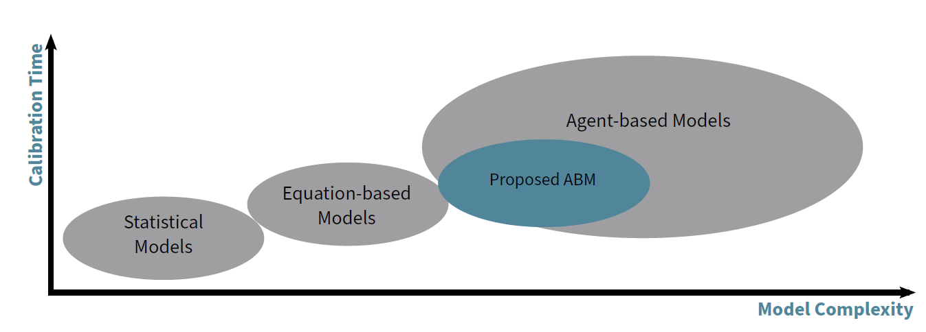
We divide the methods that are used to model the Diffusion of Innovation into three categories:
- Statistical Models: Models that find relationships between independant variables (input) and dependant variables (output). Innovation diffusion is mainly researched in the fields of Econometrics and Spatial Econometrics (Balta-Ozkan et al. 2015; Ciccarelli & Elhorst 2018; Dharshing 2017; LeSage 2015; Schaffer & Brun 2015) or by using statistical time series analysis methods (Christodoulos et al. 2010). The advantages of these models are the possibility to draw direct conclusions upon the dependencies of the output from the input variables using well known methods.
- Equation-based Models: Models where the aggregated behavior is formulated in a top-down manner using (differential) equations. The Bass Model is one example, but other approaches exist as well (Meade & Islam 2006). Those models can be calibrated with Nonlinear Least Squares Estimation (Jukić 2011; Srinivasan & Mason 1986) or Maximum Likelihood Estimation methods (Schmittlein & Mahajan 1982). The advantages of these models are that they are specifically designed to model the Diffusion of Innovations and intrinsically produce s-shaped adoption curves. Additionally, methods to calibrate those models are well established (Bemmaor & Lee 2002).
- Agent-based Models: Models where the behavior of single agents is formulated in a bottom-up manner. The system dynamics emerges from summing up individual contributions. The advantages of these models are their huge variability and extensibility, because new rules for agent behavior can easily be introduced by researchers. The transition from equation-based models to ABMs is smooth (Chatterjee & Eliashberg 1990): The Bass model, for example, can also be expressed as a simple ABM (Holanda et al. 2003; Kiesling et al. 2012) Since our work lies within this category, we will describes existing approaches in more detail within the next section.
In Figure 1 we arrange the three categories according to their complexity and calibration effort and place the our proposed ABM within this context.
ABMs of innovation diffusion
The question of what is an agent-based model is not easy to answer, since the term ABM lacks a common definition. Macal (2016) offers different ideas of what can become a general definition. He proposes ABMs to be models where agents are represented individually with diverse characteristics, and he proposes that ABMs can have autonomous agents that interact with others and the environment. Empirically grounded ABMs are ABMs that are parameterized, initialized, or evaluated by empirical data sets (Zhang & Vorobeychik 2016). They have two features in common: (1) They rely on input data sets and (2) their output is compared to data from the real world.
In the field of modeling Innovation Diffusion with ABMs, general Reviews (Kiesling et al. 2012) and Reviews with a focus on empirically grounded models exist (Scheller et al. 2019; Zhang & Vorobeychik 2016). Johanning et al. (2020) extracted and summarized common methods and patterns from existing empirical ABMs of Innovation Diffusion. In this work, we will focus on empirical ABMs that use an utility function approach, meaning that the models introduce a term for each agent that controls the decision process. This term is usually called utility. Agents then adopt if their utility exceeds a predefined threshold.
Exemplary models with the utility function approach and an empirical background can be found in several works: Günther et al. (2011) define a utility for each agent in their study on biomass fuel diffusion. An agent wants to buy the biofuel if the utility exceeds an individual threshold. McCoy & Lyons (2014) simulate the diffusion of electric vehicles by assigning a utility to each agent. Here, the agent adopts with a certain probability as soon as the utility reaches a threshold. The weights within the utility are not calibrated to some data set but drawn randomly, where the range of possible values depends on the subgroup the agent belongs to. Kaufmann et al. (2009) show that the Theory of Planned Behavior (TBC, see Ajzen 1991; Muelder & Filatova 2018) also fits into the utility function approach. Their agents adopt if the intention value exceeds a derived threshold, where the intention is a weighted sum over the the agents attitude, subjective norm, and perceived behavioral control.
For the case of studying the diffusion of photovoltaic systems, several works use a utility function approach. Zhao et al. (2011) calculate a desire level for each agent, which is a weighted sum with four free parameters. Once again, agents adopt if the desire level becomes greater than some threshold. Instead of calibrating the weights to some data set, they decided to use a survey to find the importance of each factor for the decision process. Palmer et al. (2015) use a weighted utility sum with four terms to study the diffusion of PV systems in Italy. Those terms account for the payback period, the environmental benefit of the investment, the household income, and the influence of communication with other agents. The weights of the four terms are not equal for all agents. They depend on the Sinus-Milieu the agent was assigned to. To calibrate their model and find a good threshold value, they run the ABM several times and choose the parametrization that produces the best results. Pearce & Slade (2018) base their utility on agents’ income, the decision of neighboring agents, the capital cost, and the payback period of the investment. Similar to most other models, agents adopt if their utility exceeds a threshold. To find values for the five free parameters (four weights and the threshold value), they used the method of Approximate Bayesian Computation and ran their model 500,000 times on the High Throughput Computing facility of the Imperial College High Performance Computing Service. Schiera et al. (2019) use the Theory of Planned Behavior, where agents adopt if their behavior is greater than a user-defined threshold. The behavior is a weighted sum over the Behavioral Intention (bi) and the Perceived Behavioral Control (pbc), where both bi and pbc are weighted sums on its own. The values for the weights are found by a parameter swipe with a much smaller model of a "dummy city". In their conclusion, they write that the "main limitation of the presented work is most likely in the calibration of the ABM model".
In a theoretical work on the dependence of Innovation Diffusion on network topology, Delre et al. (2010) define agents that adopt if they have been informed about the Innovation and if their utility is higher than some threshold. We mention this work here even though it uses two steps within the decision process since agents first have to check their information status. But as we will discuss at the end of 1.1.3 Section 3, an information barrier could also be included in the utility function which avoids the first step in the decision process. McCullen et al. (2013) also contribute a theoretical work and test the influence of utility weight values and network topology on the outcome of the simulation.
Regarding the TBC, Muelder & Filatova (2018) summarize different approaches of merging the TBC and ABMs. Their finding is that many works translate the TBC into a multiattribute utility, and that the functional form often is a weighted sum.
When calibrating their models to empirical data, all of the above mentioned works do not make use of model gradients. Instead they compare model outputs from different parameters to empirical data using some kind of distance function. To find good parameter values without knowing the gradients, methods from the well researched field of black-box function optimization are used (Lamperti et al. 2018; McCulloch et al. 2022; Seri et al. 2021; Shan & Wang 2010). The advantage of the black-box function methods lies at hand: Since they do not require any knowledge about the model, the same methods can be applied to a variety of different models. A good comparison on gradient-free calibration of ABMs can be found in Platt (2020) and Carrella (2021). On the other hand, a gradient-based calibration is model-specific. If the model changes, the gradients change and the calibration algorithm has to be adapted. Their advantage however is a more efficient model calibration, since they can make use of model-internal knowledge during the calibration.
Our contribution to the field of simulating the Diffusion of Innovations with ABMs is the following: We first have identified a common method already used in literature, the utility function approach. This method is formulated by us in a generalized way in Section 3. Afterwards we show that the model is differentiable. Hence, it can be efficiently calibrated using gradient-based approaches (Lee et al. 2018). We then calculate the gradients and apply a gradient-based calibration in one test case.
Model
In the beginning of this section, we will discuss the input and output of an empirical ABM of Innovation Diffusion (Figure 2, left and right boxes). Inputs to an ABM are independent of the modeling procedure. They consist of external data sets and the model initialization. External data is highly relevant if the model aims to reproduce empirical data (Salgado & Gilbert 2013). As an example, if one is investigating the diffusion of a new product and there are regions where agents are wealthier, more of them might buy the new product. Therefore, a data set of income or wealth is helpful for the model to produce good results. If there is no data available, one can also use submodels to produce the desired attribute. If one knows the average income in a region, a very simple submodel could assign an income to each agent according to a general income distribution which has the known mean value. The performance of an empirically grounded ABM is always limited by the quality of the explanatory data, so researchers have to identify the relevant data sets.
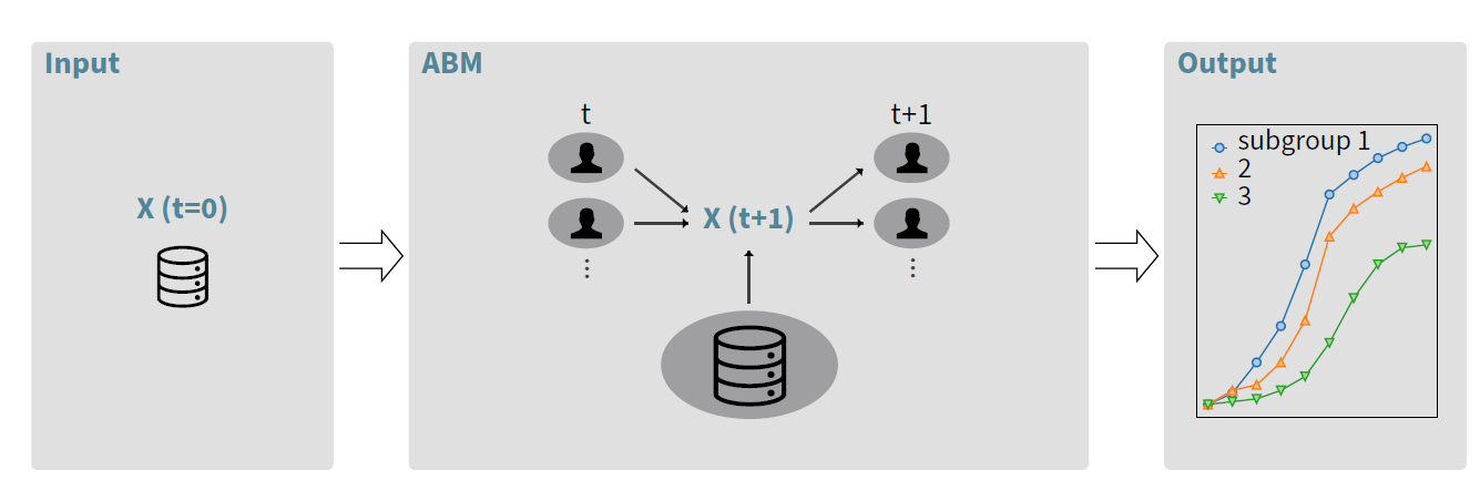
The output of the ABM is a single or multiple adoption curves, which show the number of agents that have adopted the innovation over time. When agents are divided into subgroups based on common attributes (for example, agents from different towns, different ages etc), we can also see the collection of adoption curves from subgroups as the intentional output. This output is then compared to real-world adoption data.
As pointed out in Section 2, many works use a similar method to simulate the Diffusion of Innovations with ABMs which we have called utility function approach. We’ll now describe this method in a general form following the ODD protocol (Grimm et al. 2006).1
The purpose of the presented ABM is the simulation of Innovation Diffusion. Its goal is to produce the adoption curves for different subgroups. Therefore, individual consumers who can adopt the innovation are identified as agents. Agents are characterized by their binary adoption state, which is \(1\) at time \(t\) if the agent adopts at that point in time. The decision process that is responsible for the adoption is described in the next section.
The attribute vector \(\vec{X_n}(t) \in \mathbb{R}^{M}\) of agent \(n\), where \(M\) is the number of different attributes, is the only quantity that influences the agent’s decision to adopt. Some of those attributes come from the input data and are already defined for all timesteps at the beginning of the simulation. For example, a data set of the income of agents over time can become one attribute. In Figure 2, the immutable parts of the agent attribute are represented by the database icon. In contrast to that, the attributes can also depend on the simulation. The number of adopters in the neighbourhood of an agent is often used in ABMs. This attribute is initialized at \(t=0\) and then calculated at each time step from the adoption status of the neighboring agents. In general, the attributes of an agent are influenced by the agent itself, by other agents and by the empirical data. We concatenate the attributes of all agents to get the attribute matrix \(X(t)\in \mathbb{R}^{M \times N}\), where \(N\) is the total number of agents. The model then simulates the adoption decisions and keeps track of the binary adoption state of each agent over a given number of discrete time steps.
Decision process
Let us now take a closer look at the decision process of a single agent \(n\), which is schematically shown in Figure 3. The decision of the agent at time \(t\) to adopt the innovation and hence to change its adoption status from \(0\) to \(1\) is only influenced by the attributes \(\vec{X}_n(t)\). The attributes of agent \(n\) are the input for the utility function
| \[ u_{n,t} = u \left( \vec{X}_n(t),\vec{\alpha} \right) \; \in \mathbb{R},\] | \[(1)\] |
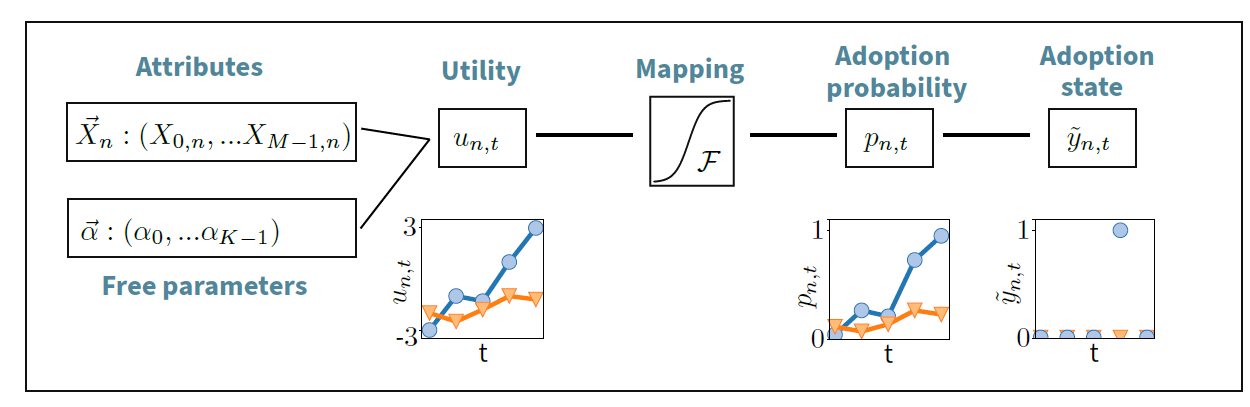
The utility \(u_{n,t}\) is then mapped to an adoption probability \(p_{n,t}\) by using a mapping function \(\mathcal{F}\):
| \[p_{n,t}=\mathcal{F}(u_{n,t})\] | \[(2)\] |
| \[\mathcal{F}: \mathbb{R} \to [0,1]\] | \[(3)\] |
| \[\lim_{u_{n,t} \to -\infty} \mathcal{F}(u_{n,t})=0 \;\;\; \text{and } \;\;\; \lim_{u_{n,t} \to \infty} \mathcal{F}(u_{n,t})=1\] | \[(4)\] |
| \[\frac{\partial}{\partial u_{n,t}}\mathcal{F} \geq 0 \;\;\; \forall u_{n,t} \in \mathbb{R}\] | \[(5)\] |
Having an adoption probability, we continue by defining an adoption variable
| \[ \tilde{y}_{n,t} = \begin{cases} \ 1 &\text{ if } \ \ \ \tilde{y}_{n,t'}= 0 \ \ \ \forall \ t'<t \ \ \text{ and } \ \ p_{n,t} > p \\ \ 0 & \text{ else.} \end{cases}\] | \[(6)\] |
Often it is pointless to consider the adoption behavior of every single agent, especially if the available data is not detailed enough. Building a model that predicts the time of adoption of each agent will probably fail when investigating many agents, but building a model that aggregates the decisions of agents in subgroups can be successful (Henry & Brugger 2017). To which subgroup an agent belongs can be defined by the agent’s location, age, or comparable characteristics. Being able to define subgroups of agents in the model is especially useful to model spatiotemporal data. The number of new adopters at time \(t\) in the \(g\)th subgroup:
| \[ \tilde{Y}_{g,t}(\vec{\alpha}) = \sum_{n\ \in \ G} \tilde{y}_{n,t}(\vec{\alpha}) \; \in \mathbb{N}_0\] | \[(7)\] |
The utility function
In the social sciences, a variety of theories explain individual decisions (Schlüter et al. 2017). For modelers, it is challenging to break down those qualitative theories into a quantitative model. Since we did not predefine the utility function in Equation 1, we keep our ABM as general as possible and give modelers the possibility to implement their interpretations of qualitative theories. Their concretization of the utility function \(u_{n,t}\) becomes the core of the adoption model and the lever controlling the simulation’s complexity. However, to utilize our ABM, it is crucial that the social science theory can be broken down to a one-step calculation of an agent’s utility. In the following, we will highlight and discuss one possible realization of \(u_{n,t}\).
A rather simple form of the utility can be obtained by introducing one free parameter per agent’s attribute and then summing over all attributes multiplied with the corresponding free parameter:
| \[\begin{aligned} u_{n,t}=\sum_{m=1}^M \alpha_m X_{m,n}(t)\end{aligned}\] | \[(8)\] |
| \[\begin{aligned}\dfrac{\partial}{\partial \alpha_k} u_{n,t} = X_{k,n}(t) \end{aligned}\] | \[(9)\] |
In the section on ABMs of Innovation Diffusion, we have already seen works that use a weighted sum as the agent’s utility. Some of those ABMs introduce an income barrier, only allowing agents with an income higher than some threshold to calculate an adoption probability. Those approaches include a "two-step" calculation of the utility and seem incompatible with our general ABM, but notice that they are actually included. This can be seen by adding a large negative term \(D \cdot H(\theta-I_n)\), where \(I_n\) is the income of agent \(n\), \(\theta\) is the income threshold, \(H(x)\) is the Heaviside step function and \(D\) is a large, negative number. By doing so, agents that have an income smaller than \(\theta\) have a large negative utility and will not adopt the innovation.
The weighted sum is of course only one of many possible forms of the utility function. Nonlinearities can be introduced by changing the functional form or by introducing additional parameters, for example, as exponents of attributes (Kahneman & Tversky 2013).
Gradients of the Model
In this section, we will introduce a loss function that measures the quality of the model prediction. We will then explicitly calculate the gradients of that loss function with respect to the free parameters \(\alpha_k\) and analyze the different terms of the gradient and their importance. A link to a python implementation of the gradients can be found in Section 9.
To empirically ground the model, the free parameters \(\vec{\alpha}\) in Equation 3 need to be calibrated to some data set. Therefore, a measure is needed that tells us how well the model performed. We will use the sum of squared residuals and introduce it as a loss function:
| \[ L = \; \sum_{g,t} \; \left( Y_{g,t} - \tilde{Y}_{g,t}(\vec{\alpha}) \right) ^2,\] | \[(10)\] |
In Equation 5, we see that \(L\) is a function of the random variable \(\tilde{Y}\) and therefore a random variable itself. Hence we search an expression for the gradient of the mean loss function \(\langle L \rangle\) with respect to the \(k\)th free parameter \(\alpha_k\). For a better readability, the dependencies on time \(t\), subgroup \(g\) and parameter \(\vec{\alpha}\) are dropped where they are not relevant.
| \[\begin{aligned} \frac{\partial}{\partial \alpha_k} \; \langle L \rangle \;\; &= \;\;\frac{\partial}{\partial \alpha_k} \langle \sum_{g,t} \; \left( Y - \tilde{Y} \right) ^2 \rangle = \; \text{-}2 \sum_{g,t} \; \langle \; \left( Y - \tilde{Y} \right) \cdot \frac{\partial}{\partial \alpha_k} \tilde{Y} \; \rangle = \; \text{-}2 \sum_{g,t} \left( \langle Y \frac{\partial}{\partial \alpha_k} \tilde{Y} \rangle - \langle \tilde{Y}\frac{\partial}{\partial \alpha_k}\tilde{Y} \rangle \right) \nonumber \\ & = \; \text{-}2 \sum_{g,t} \left(Y \frac{\partial}{\partial \alpha_k} \langle \tilde{Y} \rangle - \frac{1}{2} \frac{\partial}{\partial \alpha_k} \langle \tilde{Y}^2 \rangle \right) \nonumber \approx \; \text{-}2 \sum_{g,t} \left(Y \frac{\partial}{\partial \alpha_k} \langle \tilde{Y} \rangle - \frac{1}{2} \frac{\partial}{\partial \alpha_k} \langle \tilde{Y} \rangle^2 \right) \nonumber \\ & = \; \text{-}2 \sum_{g,t} \left(Y - \langle \tilde{Y} \rangle \right) \frac{\partial}{\partial \alpha_k} \langle \tilde{Y} \rangle. \end{aligned}\] | \[(11)\] |
Let us take a look at the remaining derivative
| \[\begin{aligned} \frac{\partial}{\partial \alpha_k} \langle \tilde{Y} \rangle \;\; = \frac{\partial}{\partial \alpha_k} \langle \sum_{n \in G} \tilde{y}_{n,t} \rangle = \;\; \sum_{n \in G} \frac{\partial}{\partial \alpha_k} \langle \tilde{y}_{n,t} \rangle.\end{aligned}\] | \[(12)\] |
| \[ \langle \tilde{y}_{n,t} \rangle = p_{n,t} \cdot \prod_{t'<t} (1-p_{n,t'} ).\] | \[(13)\] |
To pursue the calculation in Equation 7 we need the derivative of Equation 8. We continue by calculating:
| \[\begin{aligned} \frac{\partial}{\partial \alpha_k} \prod_{t'<t} (1-p_{n,t'} )&= \; \text{-}\sum_{t''<t} \frac{\partial}{\partial \alpha_k} p_{n,t''}\prod_{t'<t,t'\neq t''} (1-p_{n,t'} ) = \text{-}\sum_{t''<t} \frac{\partial}{\partial \alpha_k} p_{n,t''}\dfrac{\prod_{t'<t} (1-p_{n,t'} )}{1-p_{n,t''}} \nonumber \\ &= \; \text{-} \prod_{t'<t} (1-p_{n,t'} ) \sum_{t''<t} \dfrac{\frac{\partial}{\partial \alpha_k} p_{n,t''}}{1-p_{n,t''}}.\end{aligned}\] | \[(14)\] |
The only task left is to evaluate the derivative of \(p_{n,t}\).
| \[\frac{\partial}{\partial \alpha_k} p_{n,t} = \frac{\partial}{\partial \alpha_k} \mathcal{F}(u_{n,t}) = f(u_{n,t}) \frac{\partial}{\partial \alpha_k} u_{n,t},\] | \[(15)\] |
| \[\begin{aligned} \frac{\partial}{\partial \alpha_k} \; \langle L \rangle \;\; & \approx \; \text{-}2 \sum_{g,t} \left(Y_{g,t} - \langle \tilde{Y}_{g,t} \rangle \right) \frac{\partial}{\partial \alpha_k} \langle \tilde{Y}_{g,t} \rangle \;\; = \; \text{-}2 \sum_{g,t} \left(Y_{g,t} - \langle \tilde{Y}_{g,t} \rangle \right) \;\; \sum_{n \in G} \frac{\partial}{\partial \alpha_k} \langle \tilde{y}_{n,t} \rangle\;\; \nonumber \\ & = \; \text{-}2 \sum_{g,t} \left(Y_{g,t} - \sum_{n \in G} \mathcal{F}(u_{n,t}) \right) \\ & \; \; \; \; \; \; \; \; \cdot \sum_{n \in G} \left[ \left( \prod_{t'<t} 1-\mathcal{F}(u_{n,t'} ) \right) \left( f(u_{n,t}) \frac{\partial}{\partial \alpha_k} u_{n,t} - \mathcal{F}(u_{n,t}) \sum_{t''<t} \dfrac{f(u_{n,t''}) \frac{\partial}{\partial \alpha_k} u_{n,t''}}{1-\mathcal{F}(u_{n,t''})} \right) \right]. \nonumber\end{aligned}\] | \[(16)\] |
Discussion of the gradient
Next, we want to discuss the meaning of the different terms within the gradient in Equation 11. For simplicity, let us assume \(\frac{\partial}{\partial \alpha_k} u_{n,t}>0\). This means that a rise in parameter \(\alpha_k\) results in a rise of the utility of the \(n\)th agent and therefore in a rising adoption probability. In the opposite case, \(\frac{\partial}{\partial \alpha_k} u_{n,t}<0\) causes a changing sign, but the overall idea stays the same. Our goal now is to understand the influence of single terms on the overall sign of the gradient.
We start our analysis by recognizing that the gradient is a sum, where every summand comes from one data point and model prediction of subgroup \(g\) and time step \(t\). The sign of each summand is influenced by the term \(Y_{g,t} - \sum_{n \in G} \mathcal{F}(u_{n,t})\). This difference is negative if the model prediction is larger than the actual data and positive else. The meaning of this is intuitive: The parameter \(\alpha_k\) grows if the predicted number of adopters in subgroup \(g\) at time \(t\) is smaller than in reality (and vice versa).
The remaining part of the gradient is more complicated and comes from the derivative of the model \(\frac{\partial}{\partial \alpha_k} \langle \tilde{Y} \rangle\). It consists of a sum over all agents that belong to the same subgroup \(G\). In general, the contributions of the agents to this sum can be either negative or positive. The sum will have a positive sign, if most of the agents in subgroup \(G\) add a positive term. In the proceeding, we focus on one agent and fix \(n\).
The product \(\prod_{t'<t} 1-\mathcal{F}(u_{n,t'})\) reflects the larger impact of the adoption behaviour at early times compared to later times. This is rather intuitive: if the adoption probability of the agent is very high in the beginning, it is very likely that the agent adopts early and the circumstances at later times do not matter anymore. Mathematically, we know that \(0<\mathcal{F}(u_{n,t'})<1\), so all the factors \(1-\mathcal{F}(u_{n,t'})\) lie also between \(0\) and \(1\). For large times \(t\), more and more factors are multiplied and the value of the product decreases.
The next term \(f(u_{n,t}) \frac{\partial}{\partial \alpha_k} u_{n,t}\) is from the simple influence of \(\alpha_k\) at time \(t\) and agent \(n\). If we only consider \(\frac{\partial}{\partial \alpha_k} u_{n,t}>0\) and remember that \(f(u_{n,t})\) is a probability density and hence always larger than 0, we see that this term is positive. It tells us that an increase of \(\alpha_k\) results in an increase of the utility and more agents will adopt.
The second term, which includes the sum over \(t''\), represents the influence of \(\alpha_k\) on the group of non-adopters at time \(t\). If agent \(n\) has already adopted at earlier times, it cannot adopt at time \(t\). Thus, if the model needs to predict a larger number of adopters at time \(t\), it eventually has to reduce the value of \(\alpha_k\) so that enough non-adopters remain at later times. Once more, with the assumption of \(\frac{\partial}{\partial \alpha_k} u_{n,t}>0\) this term is always negative. Thus, the two terms in the last bracket have opposite signs. The sign of the summand of the \(n\)th agent depends on which of the two terms is larger.
Having discussed the different terms within the gradients, we turn our focus to the two specifications of \(\mathcal{F}\): (1) By choosing \(\mathcal{F}=\dfrac{1}{2}\left[1+\text{erf}\left( \dfrac{u_{n,t}}{\sqrt{2}\sigma}\right)\right]\) we get a Gaussian Model (since this chosen \(\mathcal{F}\) is the CDF of the gaussian distribution) and (2) by setting \(\mathcal{F}=H(u_{n,t})\) with \(H(u_{n,t})\) being the Heaviside step function we get a deterministic Threshold Model. The Gaussian Model has smooth gradients and will be used later in our work when testing the ABM on the data set of PV diffusion in Germany. The Threshold Model on the other side is already applied in many of the papers summarized earlier in this work. For this reason, we want to mention it explicitly as one specification of the ABM.
For the Gaussian Model, the gradient in Equation 11 is exact up to the approximation in Equation 6. In the deterministic Threshold Model, the probability density function \(f\) appearing in all summands of the gradient is the Dirac delta function \(\delta(u_{n,t})\). It is only nonzero for \(u_{n,t}=0\). This results in the gradients being zero, which makes the optimization impossible. Since the Threshold Model appears quite often in recent studies, an effective calibration method for this model is of special relevance. We bypass the problem of vanishing gradients by setting the probability distribution function \(f(u_{n,t})=1\) in the gradient of the Threshold Model. The strongest argument supporting this idea is the fact that those approximated gradients can be used to achieve good results comparable to the Gaussian Model in Section 5.
Additionally, we bring up the subsequent argument for setting \(f=1\) in the Threshold Model. In the head or center region, the probability distribution is of order \(1\). In this region, the CDF has the steepest slope and a change in free parameters (and the resulting change in the utility) strongly influences the adoption probability of an agent. In the tail of the distribution, \(f\) is much smaller than \(1\). Here, a change in the free parameters does not really affect the agent’s behavior. This is normally reflected by \(f \approx 0\), which suppresses the influence of this specific agent on the gradient. In the case of the Threshold Model, only agents with a utility infinitesimal close to the threshold value of \(0\) change their behavior for a change in the utility. Those agents are extremely rare. By setting \(f=1\), all agents equally contribute to the gradient, even though their behavior is not affected by a small change in the parameters. This should result in the gradient of the Threshold Model being much larger, but the direction of the gradient still should be right. The large gradient is one reason why the choice of the advanced gradient-based optimizer Adam will be important later on. Vanilla gradient descent will in general have many problems in handling those large gradients. In conclusion, we are not able to confirm this argument mathematically due to the complex nature of the gradients. The only justification for setting \(f=1\) is the strong calibration results, which is an indication that the idea is right.
Finally, we also want to discuss the differentiability of the utility function in Equation 4. It is important to mention that the gradient in Equation 4 is only valid if the input variables do not depend on the model outcome (and are therefore independent of \(\alpha_k\)). This is not a problem if \(X_k\) is an external data set, such as the income of the agent. However, it becomes a problem for variables depending on the model. Imagine that we want to use the number of adopters in the subgroup as a factor influencing the adoption decision, often referred to as peer pressure. Then, \(X_{k,n}(t)\) depends on the model output from earlier times, namely the number of adopters in the specific subgroup and hence it depends on \(\vec{\alpha}\). In this case, the gradient in Equation 4 would include a very complex term \(\alpha_k \frac{\partial}{\partial \alpha_k}X_{k,n}(t)\). One has three possibilities to handle this term. Either one can derive an expression, one finds an approximation for the derivative to keep the gradients as exact as possible, or one neglects the term. For the latter, special attention has to be paid to the convergence of the calibration, because the gradients are not exact anymore. It is also possible to calibrate the model with the imprecise gradients until it converges to a specific solution, followed by a random search around that solution. By doing so one can check if better results are in the close vicinity. Since the specific form of such complex terms depends on the model specifications, it is irrelevant for further investigations of the general ABM. Note however that we neglect a complex term \(\alpha_k \frac{\partial}{\partial \alpha_k}X_{k,n}(t)\) in the gradient for three attributes in Section 5 and still get a satisfyingly result.
Results
To test the calibration with gradients, we will model the data set of small-scale photovoltaic adoption in Germany from \(2000-2016\). The model will be calibrated to match the number of new adopters in the 401 districts of Germany at 17 consecutive years. Special attention is paid to the convergence of the calibration and the quality of the fit. First, we will compare the gradient-based calibration with two gradient-free calibration methods. Second, we will evaluate the prediction of the calibrated ABM.
Works that use ABMs in the field of Innovation Diffusion often have difficulties when calibrating their models (Rand & Stummer 2021;Zhang & Vorobeychik 2016). Traditional approaches utilize black-box function optimizers, where the gradients of the function are not needed. However, gradient-free optimization has strong difficulties with both computationally expensive functions and high-dimensional parameter spaces. For a growing number of free parameters, the usage of gradient-based calibration becomes the only method that ensures good fitting results for large models within a finite computational time (Shan & Wang 2010).
To show this, we test both a gradient-based and two gradient-free calibration methods on the dataset \(Y(g,t)\) of privately owned photovoltaic systems diffusion in Germany. The data set of small-scale photovoltaic systems is chosen for the following two reasons. First, it consists of trustworthy data on a detailed time and location level (Netztransparenz 2019). Second, by restricting ourselves to small-scale photovoltaic systems with capacities \(<10 \ \mathrm{kW_p}\) we assume that most of the decisions are not made by professional investors and that many reasons besides economic profit play a role. The diffusion of PV systems is of special relevance in the research community, since it plays an important role in the transition towards a renewable energy system (Zhang & Vorobeychik 2016).
The data set \(Y(g,t)\) consists of \(6817\) data points, each representing the number of adopters in one specific district \(g\) and one year \(t\). The chosen model utility is a weighted sum as in Equation 4 with \(25\) free parameters and \(\mathcal{F}\) is the CDF of the gaussian distribution, so that we end up with the Gaussian Model as described in Section 4. The largest model used during the calibration consists of \(1.6\) million agents. A detailed description of the PV diffusion model and its input data can be found in the appendix.
Our procedure is as follows. We run our model with an initial set of free parameters \(\vec{\alpha}_0\). This produces an adoption prediction of the model \(\tilde{Y}(g,t,\vec{\alpha}_0)\). The quality of the model output is determined via the loss function \(L\) in Equation 5. Our ultimate goal is to minimize \(L\) by changing the free parameters \(\vec{\alpha}\) during the calibration. From the variety of possible calibration methods (Carrella 2021; Salle & Yıldızoğlu 2014) we decided to test Bayesian optimization and Direct Search optimization as two gradient-free methods before applying a gradient-based approach.
Bayesian optimization
Bayesian optimization is a machine-learning surrogate optimization method used to optimize expensive black-box functions. The method is well suited, if the dimension of the parameter space is not too large (typically \(\leq 20)\), the objective function is continuous, expensive to evaluate and has no first- or second-order derivative. Bayesian optimization then aims at finding a global optimum of the objective function.
In a surrogate method, the expensive-to-evaluate objective function is replaced by a surrogate function. During the optimization, the algorithm calculates a function estimate together with a confidence interval. The parameters for the next function evaluation are then chosen with the help of the surrogate. For a detailed description of the method, we refer to Frazier (2018).
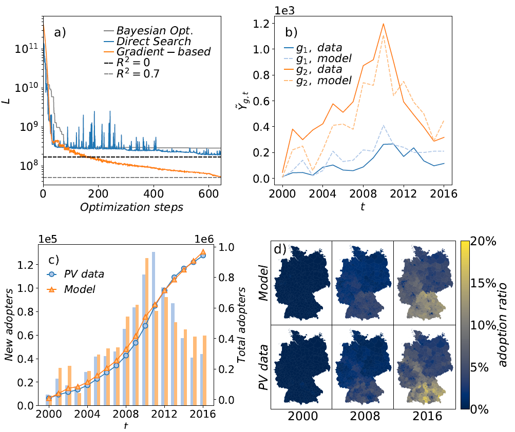
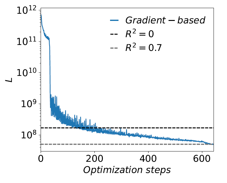
When used to calibrate the ABM on the data set of PV diffusion, Bayesian optimization does not perform well (see Figure 4a). After \(700\) optimization steps, the best model achieves \(L \approx 2.8 \cdot 10^8\), which corresponds to \(R^2 \approx -0.7\). The explanation for the bad result is the large dimensionality of the parameter space. The number of necessary function evaluations grows exponentially with the number of free parameters and thus a method that aims to find a global minimum by examining the whole parameter space is not suited for the calibration of this expensive-to-evaluate ABM that contains 25 parameters.
Direct search optimization
The next gradient-free calibration method we use is a Direct Search method. In this method, a random starting point is chosen and the behavior of the function in the neighborhood is evaluated. If the function decreases in one direction, we follow this direction (Kolda et al. 2003). In the case of calibrating the ABM, we need an algorithm that can handle noisy functions and therefore use a search optimizer from the Python package noisyopt (Mayer et al. 2016).
When calibrating the Gaussian Model with the direct search optimizer, the achieved \(R^2\) is still smaller than \(0\) after \(650\) steps (see Figure 4a, blue curve), hence the fit is still worse than simply taking the mean of the data. To save computational time, the pattern search algorithm was performed on a reduced model with roughly \(640,000\) agents.
With a Direct Search algorithm, we no longer aim to find a global minimum and hence do not have to scan the exponentially increasing parameter space. However, the convergence of the algorithm to some local minimum is still very slow. This can once again be explained by the high dimensionality of the parameter space, which slows down the evaluation of the local neighborhood.
Gradient-based optimization
The gradient-based optimization is performed with the Adam optimizer (Kingma & Ba 2014) which needs the first-order derivative calculated in Section 4. Compared to vanilla gradient descent, Adam has the advantage of faster convergence due to its adaptive learning rate, the ability to escape local minima, and the ability to handle stochastic functions. The optimization ends after a given number of steps.
To reduce the computational time in the gradient-based calibration, we start with a relatively small model with few agents, and enlarge the model during the optimization process. The idea is that the rough direction of the gradients can also be calculated with a small model, especially if the calibration process has not yet advanced far from its random starting point. Only later on, a large model is needed to further improve the fitting result. We start the calibration with \(\sim 16,000\) agents, where each agent represents \(1,000\) privately owned households, and increase the model during the calibration up to the value of \(1.6\) million agents, where each agent represents \(10\) households.
The result can be seen in Figure 4a. The ABM can be fitted to \(R^2 \simeq 0.7\) with the gradient-based Adam Optimizer. For the first \(600\) steps, the number of agents in the model is increased linearly up to \(640,000\) agents. For the last steps, a larger number of agents is added per step, which explains the small bend of the curve. The model size used for the gradient-free direct search method is passed for the gradient-based optimization at the \(600th\) step, where the quality of the fit is already above \(R^2=0.6\).
We also want to add that we tested the gradient-based calibration on the Threshold Model as well. In the Threshold Model, the gradients are not exact as we have discussed in Section 4. Nevertheless, the calibration result is equally good with \(R^2 \simeq 0.7\) and can be found in the Appendix.
Evaluation of the calibrated ABM
Next, we want to evaluate the ABM that was calibrated with the gradient-based Adam optimizer and compare it to the PV data set. In Figure 4b, both \(Y_{g,t}\) and \(\tilde{Y}_{g,t}\) are shown for two of the 401 districts. We see that the model output (dotted line) is quite close to the actual data. In Figure 4c, the number of total adopters (lines) and the number of new adopters (bar) are shown for each year for Germany, which is the sum of \(Y_{g,t}\) over all districts. Since the calibration occurs on the level of single districts, in Figure 4d the ratio of agents that have adopted is shown for all districts for the years \(2000\), \(2008\) and \(2016\), where the ratio of adopters is defined as \(q_{adopt}=\frac{N_{adopt}}{N_{total}}\). It can be seen that the model catches all relevant spatial and temporal patterns quite well.
Discussion
The topic of validation and overfitting a model was not discussed in this work. The reason for this is that the focus of the work lies on calibrating ABMs of Innvovation Diffusion with gradients. Validating a model, however, depends on the specific model and data set. We still want to emphasize that the prevention of overfitting is of immense importance, especially when there is no upper limitation for choosing the number of free parameters. It is necessary to match the number of parameters to the size of the empirical data set and to spend time on validating the specific model, either by using cross-validation or other techniques (Fagiolo et al. 2019; Miller 1998).
Possible applications of the proposed ABM
To identify fields where the ABM of Innovation Diffusion can be applied, we shortly summarize the two main aspects of the ABM:
- The focus of the model lies on the decision of agents to adopt, which is manifested in the change of the adoption variable \(\tilde{y}\). An agent can only adopt once and stays an adopter then.
- The decision process of an agent only depends on the differentiable utility function \(u_{n,t}\). Decision processes that are more complex can not be included.
For the evaluation of PV systems diffusion, we delivered one example where the ABM can be applied. At least for smaller time horizons, one can fairly say that people who bought a PV system still own this system and neglect the number of deconstructions. Hence we fulfill the requirement that agents can only adopt once and that they stay adopters afterwards. A counter example, where the ABM can not be applied, is to use the ABM to simulate the number of agents that own a car. This is due to the fact that in a data set of car owners, people appear who once owned a car in the past, but sold it. We then used a linear sum as utility function which is probably the simplest example for a differentiable function and fulfills the second requirement.
We also want to stress the drawback of the gradient-based calibration method: While other researchers worked on improving the calibration of ABMs on a very general level (Carrella 2021; Lamperti et al. 2018; Platt 2020), our method is only applicable in the described ABM of Innovation Diffusion and can make no statement about other types of models. Additionally, to use gradients, the ABM has to be rather simple and no complex decision rules for the agents are possible. While this seems applicable for the problem of Innovation Diffusion, other fields where ABMs are used need more complex models.
Regarding the question of when to use the ABM or when to use other methods, we make the following recommendation: If the goal is to find relations between input and output quantities, we recommend to use statistical methods. If the goal is to make a forecast and the microscopic view is not of interest, equation-based models are the method of choice. If a detailed bottom-up view is of interest, the proposed ABM together with its gradient-based calibration will be an appropriate choice.
Conclusion
In this work, we described a gradient-based calibration method for ABMs of Innovation Diffusion that can efficiently calibrate models with many free parameters in large-scale simulations. Traditional approaches in this field are restricted to using black-box function optimizers for model parametrization. Our general ABM together with its gradients enables researchers to empirically ground models with many parameters on large data sets. This is an important step to scale up ABMs and model Innovation Diffusion on large scales, such as the country or even global level.
In the beginning of this work, we identified a common method to simulate the Diffusion of Innovations with ABMs in literature and formulated this method in a general ABM. We then discussed the importance of the utility function with special reference to its differentiability. We highlighted the cases where the restriction of a differentiable utility function causes difficulties and how this can be handled.
Thereafter, we calculated the gradients of the general ABM which are needed to efficiently calibrate the model and discussed the meaning of the different terms appearing in the gradients. We showed that the new calibration method achieves much better results than gradient-free approaches. In contrast to these gradient-free approaches, the new method is able to produce good fits even in the case of many free parameters.
Finally, we tested the calibration technique on the data set of privately owned photovoltaic systems in Germany between \(2000-2016\). We achieved a coefficient of determination \(R^2 \simeq 0.7\) by calibrating a model including \(1.6\) million agents to more than \(6000\) data points using \(25\) free parameters. In the discussion section, we made recommendations on when and when not to use the ABM for simulating the Diffusion of Innovations.
In future works, the ABM can be applied to model other diffusion processes. The calibrated parameters can be analyzed to gain information about the influence of different agent attributes. A calibrated ABM can then be used to make predictions about future diffusion pathways.
The formulated ABM togther with its gradients enables researchers to create empirically grounded models of Innovation Diffusion with many free parameters that can be calibrated to large data sets. Simplifications to reduce the computational time of the calibration process, such as a prior fixation of some parameters or a reduced number of agents, are not obligatory anymore.
Model documentation
This work is accompanied by an implementation of a toy model and its gradients in Python that can be customized for own purposes. The Python notebook together with a step by step description can be found on GitHub: https://github.com/FlorianK13/ABM-Calibration.Acknowledgment
We want to thank Soner Candas and Smajil Halilovic from the chair of Renewable and Sustainable Energy Systems at TUM for fruitful discussions and their insightful comments on the topic of agent-based modeling and on the expansion of photovoltaic systems in Germany. Additionally, we thank Valentin Leeb for the discussion of the mathematical parts of this work and to Martin Grosshauser for proofreading. Finally, we also want to thank the three anonymous referees for their contributions in increasing the quality of this work.Notes
Since we describe a general method and not a specific ABM, some aspects of the ODD are not applicable↩︎
Appendix
The ABM together with its gradients can be used for a wide range of applications and is not limited to any special technology. However, to test the method, the ABM has to be applied to model the diffusion of a concrete technology. We chose to model the diffusion of PV systems in Germany. The model specifications, the empirical data sets, and the submodel of opinion formation that we used will be explained in detail in the following sections. In the last part, we show the parameters that were found and discuss the convergence of the optimization process.
PV diffusion model
In this section, we first explain the data set of the PV systems diffusion in Germany and the explanatory data sets. This is followed by a description of the ABM specifications for the PV diffusion model. The description contains all relevant information to reproduce the presented results. Since the focus of our work lies on the ABM and calibration method, we do not discuss the PV diffusion model and do not justify any predefined parameter values. The only purpose of the presented PV diffusion model is to test our calibration technique.
Data
The data set we want to model contains the number of PV installations of capacity \(<10\) \(\mathrm{kW_p}\) for each district (NUTS3-region) in Germany in each year \(2000-2016\), so \(Y \in \mathbf{R}^{401 \times 17}\), with 401 districts and 17 years. It is obtained from the Anlagenstammdaten, a database published by the German Federal Network Agency (Netztransparenz 2019). From this data set, all installations with a capacity \(<10\) \(\mathrm{kW_p}\) together with their municipality keys and the year of installation are extracted.
We use each privately owned household as a potential candidate for adopting a PV installation. Hence we make two approximations. First, we neglect that other types of buildings, such as apartment houses or commercial buildings can install these small systems as well. Second, households in private property could also install systems with a larger capacity and are not restricted to small systems. Both approximations are necessary due to the limited information in the available data. The number of households in private property for each district is obtained from the census data set (Zensus 2011). Overall, a total number of \(\sim 1.6 \cdot 10^7\) houses in Germany are in private property, which all are assumed to be candidates for installing a small PV system. After the time horizon of \(17\) years, roughly \(10^6\) PV installations with a capacity \(<10\) \(\mathrm{kW_p}\) exist in Germany. We assume that each PV installation can be matched to one household and therefore about 6 % of the households in Germany became an adopter.
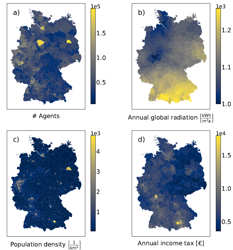
Various temporal and spatial explanatory data sets are used to model the PV adoption (see Figure 5 and Table 1). The feed-in tariffs are taken from the German Bundesnetzagentur (BNetzA 2020). The capital cost per \(\mathrm{kW_p}\) of installed capacity is from BSW Solar (BSW-Solar 2016). Electricity retail prices come from the German Federal Statistical Office (Destatis 2020). The time series on lending interest rates (Bundesbank 2020b) and deposit interest rates (Bundesbank 2020a) are from the German Bundesbank. The spatial data of the annual global radiation is from the open data collection of the public German weather administration Deutscher Wetterdienst (DWD 2020). To decrease fluctuations in the global radiation, the data is averaged over the years \(2015\) to \(2019\). The population density of each district is calculated from the census data set and the area of each district, taken from the Federal Statistical Office of Germany (Destatis 2019), which is also the source of the average income taxation per head within each district (Regionalstatistik 2016).
Following Candas et al. (2019), we use a Net Present Value \(NPV_{n,t}\) as the economic profitability , which is the expected profitability per installed \(\mathrm{kW_p}\).
| \[ NPV_{n,t}=-\ \mathrm{CC}(t) \ \mathrm{af}(t) \ t_{life} \ + \ \sum_{\tau=1}^{t_{life}}\dfrac{\left[ \mathrm{FIT}(t)(1-\mathrm{SC}(t))+\mathrm{RP}(\tau)\mathrm{SC}(t)\right] \cdot E_{rad} \cdot \eta \cdot A_{kWp}}{(1+r_{dep}(t))^\tau},\] | \[(17)\] |
| \[af(t)=\dfrac{r_{lend}(st)(1+r_{lend}(t))^{t_{life}}}{(1+r_{lend}(t))^{t_{life}}-1}\] | \[(18)\] |
| Year | Capital Cost (€/\(\mathrm{kW_p}\)) | Feed-in Tariff (ct€/kWh) | Retail Price (ct€/kWh) | Lending & Deposit rate (%) | Self-Consuption(%) | |
| \(2000\) | \(8821\) | \(66.66\) | \(18.17\) | \(6.86\) | \(2.65\) | \(0\) |
| \(2001\) | \(8017\) | \(65.36\) | \(18.98\) | \(6.89\) | \(3.03\) | \(0\) |
| \(2002\) | \(7190\) | \(61.22\) | \(19.49\) | \(6.48\) | \(1.70\) | \(0\) |
| \(2003\) | \(7496\) | \(57.57\) | \(20.22\) | \(5.39\) | \(2.40\) | \(0\) |
| \(2004\) | \(6666\) | \(71.15\) | \(20.66\) | \(5.15\) | \(2.03\) | \(0\) |
| \(2005\) | \(7451\) | \(66.56\) | \(21.18\) | \(4.56\) | \(1.37\) | \(0\) |
| \(2006\) | \(5491\) | \(62.25\) | \(21.63\) | \(4.29\) | \(0.88\) | \(0\) |
| \(2007\) | \(4869\) | \(57.81\) | \(22.53\) | \(4.64\) | \(1.26\) | \(0\) |
| \(2008\) | \(4592\) | \(53.51\) | \(21.48\) | \(5.04\) | \(0.74\) | \(0\) |
| \(2009\) | \(3405\) | \(49.08\) | \(22.82\) | \(4.73\) | \(2.78\) | \(0\) |
| \(2010\) | \(2928\) | \(44.17\) | \(23.75\) | \(4.27\) | \(2.22\) | \(0.43\) |
| \(2011\) | \(2189\) | \(31.78\) | \(25.28\) | \(3.87\) | \(0.75\) | \(1.29\) |
| \(2012\) | \(1656\) | \(26.48\) | \(25.95\) | \(3.47\) | \(0.87\) | \(4.30\) |
| \(2013\) | \(1576\) | \(18.17\) | \(29.19\) | \(2.74\) | \(0.01\) | \(8.21\) |
| \(2014\) | \(1471\) | \(14.48\) | \(29.81\) | \(2.84\) | \(0.12\) | \(9.04\) |
| \(2015\) | \(1437\) | \(13.22\) | \(29.51\) | \(2.02\) | \(1.38\) | \(10.01\) |
| \(2016\) | \(1400\) | \(12.90\) | \(29.69\) | \(1.84\) | \(0.49\) | \(9.44\) |
| \(2017\) | \(1359\) | \(12.69\) | \(30.48\) | \(1.59\) | -\(0.97\) | \(10.00\) |
Opinion formation model
In the field of Innovation Diffusion, customers have various and individual motives to adopt a new innovation. The submodel of opinion formation reflects this bounded rationality. Here we will describe the opinion formation model and explain how agents can interact with each other, with nearby adopters, and with a central agent (media).
The utilized model of opinion formation is similar to the kinetic model from Toscani (2006). It can be used to model the dynamical changes in opinion among \(N\) agents. Each agent \(n\) has a continuous opinion \(w_{n,t} \in [-1,1]\). At time \(t=0\), the opinion \(\tilde{w}_n\) is randomly drawn from a gamma distribution with \(k=7\) and \(\theta=0.1\). Then we set \(w_{n,t=0}=\tilde{w}_n-1\), where the small number of opinions lying outside of the interval \([-1,1]\) are set to the mean value of the shifted gamma distribution -\(0.4\). At each time step, agent \(n\) first interacts directly with one other agent, then it interacts with its environment, and finally with the central agent.
Direct interaction
Two agents can interact directly to change their opinion. Their initial opinions \(w_{n,t},w_{n',t}\) are updated at each time step.
| \[\begin{aligned} w_{n,t+1}=w_{n,t}- \gamma P(w_{n,t})(w_{n,t}-w_{n',t})+ \ \eta D(w_{n,t})\end{aligned}\] | \[(19)\] |
| \[\begin{aligned}w_{n',t+1}=w_{n',t}- \gamma P(w_{n',t})(w_{n',t}-w_{n,t})+ \eta D(w_{n',t}),\end{aligned}\] | \[(20)\] |
Interaction with the environment
The opinion of agent \(n\) is also influenced by its environment, which is the number of new PV installations in the district. A large number of adopters in the district positively affects the opinion of other agents.
| \[ w_{n,t+1}=w_{n,t}+\gamma_{env}P(w_{n,t}) \cdot \dfrac{\tilde{Y}(g,t-1)}{N_g},\] | \[(21)\] |
Interaction with the central agent
The interaction with a central agent represents the media’s influence on the individual agent.
| \[ w_{n,t+1}=w_{n,t}- \gamma_{CA} P(w_{n,t})(w_{CA,t}-w_{n,t}),\] | \[(16)\] |
Utility function of the PV diffusion model
The specific form of the utility function is the core of the ABM. For the PV diffusion model, we chose the product \(\vec{\alpha} \cdot X\) from Equation 8. The \(M=25\) attributes are listed below.
\(X_1=NPV_{n,norm}\) is the normalized economic profitability, see Equation 17, with \(\\ NPV_{n,norm} = \dfrac{NPV_n-NPV_{n,min}}{NPV_{n,max}-NPV_{n,min}}\).
\(X_2=w_n\) is the opinion of agent \(n\).
\(X_3=NPV_{n,norm} \cdot \dfrac{w_n+1}{2}\) is a product of the normalized economic profitability and the opinion, shifted to the interval \([0,1]\).
\(X_4\) is the normalized population density of the district the agent lives in.
\(X_5\) is the normalized average income taxation per head of the district the agent lives in.
\(X_6=NPV_{n,norm} (t+1) - NPV_{n,norm}(t)\) is the difference of the normalized economic profitability at time \(t+1\) and time \(t\).
\(X_7=\sqrt{NPV_{n,norm}}\) is the root of the normalized economic profitability, .
\(X_8=\text{FIT}(t+1)-\text{FIT}(t)\) is the normalized difference of the Feed-in Tariff at times \(t+1\) and \(t\).
\(X_9\) is the ratio of agents in each district that have adopted at the previous time step \(t-1\)
\(X_{10}\ \text{-} \ X_{25}\) are \(16\) variables representing the \(16\) states of Germany. They are binaries and are \(1\) if the agent lives in the state they’re referring to. Since each agent lives in exactly one state, we know that \(\sum_{m=9}^{24}X_{m,n}=1 \ \forall n\).
Additionally, a threshold \(\theta_n\) is subtracted from the utility in both the Threshold and the Gaussian Model. The threshold \(\theta_n\) is randomly drawn from a Beta distribution \(f(x,a,b)=\dfrac{1}{B(a,b)}\cdot x^{a-1}(1-x)^{b-1}\), where \(B(a,b)\) is the euler beta function, and \(a=5\), \(b=2\) are fixed. The threshold introduces a time-independent heterogeneity among agents. In the Gaussian Model, we set \(\sigma=1\) in the mapping function \(\mathcal{F}\).
| Model | \(\alpha_1\) | \(\alpha_2\) | \(\alpha_3\) | \(\alpha_4\) | \(\alpha_5\) | \(\alpha_6\) | \(\alpha_7\) | \(\alpha_8\) | \(\alpha_9\) |
| Threshold | -\(0.18\) | \(0.77\) | \(0.34\) | -\(0.15\) | -\(0.08\) | \(0.01\) | -\(0.09\) | \(0.05\) | \(2.87\) |
| Gaussian | -\(0.20\) | \(0.64\) | \(1.73\) | -\(0.79\) | -\(0.27\) | \(0.27\) | -\(1.08\) | \(0.66\) | \(4.20\) |
Optimal parameters and convergence
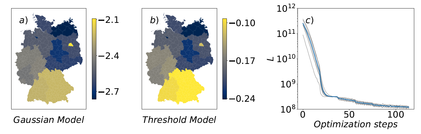
The convergence of the optimization process is highly dependant on the choice of the utility function, hence no general statements can be made for the ABM. In general, optimizers that work with the principle of gradient descent can get trapped in local minima. The Adam optimizer used in this work is able to overcome local minima, but it is not guaranteed to do so. For the PV diffusion model, we run \(8\) calibrations of a smaller model with \(320\) thousand agents. The value of the loss function \(L\) during the calibration can be seen in Figure 6, where grey lines represent single calibration processes. It can be seen that all optimizations roughly behave the same and find an equally good solution. The average distance of the final parameter vectors is \(d_{avg}= \frac{2}{N^2-N}\sum_{i,j,i\neq j} \sqrt{(\vec{\alpha}_i-\vec{\alpha}_j)^2} \simeq 1.65\). This distance is not too large, but it cannot be neglected. It shows that there is no unique solution for the parameter values for this specific PV diffusion model. We assume that this is due to the irrelevance of some of the agents’ attributes.
One set of optimal values for the free parameters of the utility in Equation 8 are presented in Table 2 and Figure 6a and b. These parameters are from a calibrated Gaussian Model with \(1.6\) million agents.
Calibration of the threshold model
The gradient-based calibration method was also tested for the Threshold Model, as the Threshold Model is predominantly used in the literature. As can be seen in Figure 7, the Threshold model also achieves \(R^2 \approx 0.7\).
References
AJZEN, I. (1991). The theory of planned behavior. Organizational Behavior and Human Decision Processes, 50(2), 179–211. [doi:10.1016/0749-5978(91)90020-t]
BALTA-OZKAN, N., Yildirim, J., & Connor, P. M. (2015). Regional distribution of photovoltaic deployment in the UK and its determinants: A spatial econometric approach. Energy Economics, 51, 417–429. [doi:10.1016/j.eneco.2015.08.003]
BASS, F. M. (1969). A new product growth for model consumer durables. Management Science, 15(5), 215–227. [doi:10.1287/mnsc.15.5.215]
BDEW (2016). Energie-Info: Erneuerbare Energien und das EEG: Zahlen, Fakten, Grafiken (2016). Available at: https://www.bdew.de/service/publikationen/energie-info-erneuerbare-energien-und-das-eeg-zahlen-fakten-grafiken-2016/.
BEMMAOR, A. C., & Lee, J. (2002). The impact of heterogeneity and ill-Conditioning on diffusion model parameter estimates. Marketing Science, 21(2), 209–220. [doi:10.1287/mksc.21.2.209.151]
BNETZA (2019). Zahlen, Daten und Informationen zum EEG: EEG in Zahlen 2019. Available at: https://www.bundesnetzagentur.de/DE/Sachgebiete/ElektrizitaetundGas/Unternehmen_Institutionen/ErneuerbareEnergien/ZahlenDatenInformationen/zahlenunddaten-node.html.
BNETZA (2020). Bundesnetzagentur: Archivierte EEG-Vergütungssätze und datenmeldungen. Available at: https://www.bundesnetzagentur.de/DE/Sachgebiete/ElektrizitaetundGas/Unternehmen_Institutionen/ErneuerbareEnergien/ZahlenDatenInformationen/EEG_Registerdaten/ArchivDatenMeldgn/ArchivDatenMeldgn_node.html.
BOERO, R., & Squazzoni, F. (2005). Does empirical embeddedness matter? Methodological issues on agent-based models for analytical social science. Journal of Artificial Societies and Social Simulation, 8(4), 6: https://www.jasss.org/8/4/6.html. [doi:10.18564/jasss.1620]
BSW-SOLAR. (2016). Photovoltaik-Preismonitor Deutschland: German PV Module Price Monitor, first quartal. German PV Module Price Monitor, first quartal. Available at: https://www.solarwirtschaft.de/fileadmin/user_upload/BSW_Preismonitor_Q1_2016.pdf.
BUNDESBANK. (2020a). Einlagen privater Haushalte, vereinbarte laufzeit von über 2 jahren. Available at: https://www.bundesbank.de/dynamic/action/de/statistiken/zeitreihen-datenbanken/zeitreihen-datenbank/759778/759778?listId=www_s510_rzmfi.
BUNDESBANK. (2020b). Wohnungsbaukredite an private Haushalte, anfängliche zinsbindung über 5 bis 10 jahre. Available at: https://www.bundesbank.de/dynamic/action/de/statistiken/zeitreihen-datenbanken/zeitreihen-datenbank/759778/759778?listId=www_s510_ph3_neu.
CANDAS, S., Siala, K., & Hamacher, T. (2019). Sociodynamic modeling of small-scale PV adoption and insights on future expansion without feed-in tariffs. Energy Policy, 125, 521–536. [doi:10.1016/j.enpol.2018.10.029]
CARRELLA, E. (2021). No free lunch when estimating simulation parameters. Journal of Artificial Societies and Social Simulation, 24(2), 7: https://www.jasss.org/24/2/7.html. [doi:10.18564/jasss.4572]
CHATTERJEE, R. A., & Eliashberg, J. (1990). The innovation diffusion process in a heterogeneous population: A micromodeling approach. Management Science, 36(9), 1057–1079. [doi:10.1287/mnsc.36.9.1057]
CHRISTODOULOS, C., Michalakelis, C., & Varoutas, D. (2010). Forecasting with limited data: Combining ARIMA and diffusion models. Technological Forecasting and Social Change, 77(4), 558–565. [doi:10.1016/j.techfore.2010.01.009]
CICCARELLI, C., & Elhorst, J. P. (2018). A dynamic spatial econometric diffusion model with common factors: The rise and spread of cigarette consumption in Italy. Regional Science and Urban Economics, 72, 131–142. [doi:10.1016/j.regsciurbeco.2017.07.003]
DELRE, S. A., Jager, W., Bijmolt, T. H. A., & Janssen, M. A. (2010). Will it spread or not? The effects of social influences and network topology on innovation diffusion. Journal of Product Innovation Management, 27(2), 267–282. [doi:10.1111/j.1540-5885.2010.00714.x]
DESTATIS. (2019). Kreisfreie städte und landkreise nach fläche, bevölkerung und bevölkerungsdichte.
DESTATIS. (2020). Daten zur Energiepreisentwicklung - Lange Reihen bis November 2020. Available at: https://www.destatis.de/DE/Themen/Wirtschaft/Preise/Publikationen/Energiepreise/energiepreisentwicklung-pdf-5619001.pdf.
DHARSHING, S. (2017). Household dynamics of technology adoption: A spatial econometric analysis of residential solar photovoltaic (PV) systems in Germany. Energy Research & Social Science, 23, 113–124. [doi:10.1016/j.erss.2016.10.012]
DWD. (2020). German meteorological service: Open data of the climate data center. at: https://www.dwd.de/DE/leistungen/cdc/climate-data-center.html?nn=16102.
EPSTEIN, J. M. (2008). Why model? Journal of Artificial Societies and Social Simulation, 11(4), 12: https://www.jasss.org/11/4/12.html.
FAGIOLO, G., Guerini, M., Lamperti, F., Moneta, A., & Roventini, A. (2019). 'Validation of agent-based models in economics and finance.' In C. Beisbart & N. J. Saam (Eds.), Computer Simulation Validation (pp. 763–787). Berlin Heidelberg: Springer. [doi:10.1007/978-3-319-70766-2_31]
FRAZIER, P. I. (2018). A tutorial on Bayesian optimization. arXiv preprint. Available at: https://arxiv.org/pdf/1807.02811.pdf%C2%A0.
GNANN, T., Stephens, T. S., Lin, Z., Plötz, P., Liu, C., & Brokate, J. (2018). What drives the market for plug-in electric vehicles? A review of international PEV market diffusion models. Renewable and Sustainable Energy Reviews, 93, 158–164. [doi:10.1016/j.rser.2018.03.055]
GRIMM, V., Berger, U., Bastiansen, F., Eliassen, S., Ginot, V., Giske, J., Goss-Custard, J., Grand, T., Heinz, S. K., Huse, G., & others. (2006). A standard protocol for describing individual-based and agent-based models. Ecological Modelling, 198(1-2), 115–126. [doi:10.1016/j.ecolmodel.2006.04.023]
GÜNTHER, Stummer, C., Wakolbinger, L. M., & Wildpaner, M. (2011). An agent-based simulation approach for the new product diffusion of a novel biomass fuel. Journal of the Operational Research Society, 62(1), 12–20.
HELBING, D. (2012). 'Agent-Based modeling'. In D. Helbing (Ed.), Social Self-Organization: Agent-Based Simulations and Experiments to Study Emergent Social Behavior (pp. 25–70). Springer.
HENRY, A. D., & Brugger, H. I. (2017). 'Agent-Based explorations of environmental consumption in segregated networks.' In C. García-Díaz & C. Olaya (Eds.), Social Systems Engineering (pp. 197–214). John Wiley & Sons. [doi:10.1002/9781118974414.ch10]
HESSELINK, L. X., & Chappin, E. J. (2019). Adoption of energy efficient technologies by households–barriers, policies and agent-based modelling studies. Renewable and Sustainable Energy Reviews, 99, 29–41. [doi:10.1016/j.rser.2018.09.031]
HOLANDA, G. M., Bazzan, A. L., Gerolamo, G. P., Franco, J., & Martins, R. (2003). Modeling the Bass diffusion process using an agent-based approach. Workshop on Agent-Based Simulation.
JOHANNING, S., Scheller, F., Abitz, D., Wehner, C., & Bruckner, T. (2020). A modular multi-agent framework for innovation diffusion in changing business environments: Conceptualization, formalization and implementation. Complex Adaptive Systems Modeling, 8(1). [doi:10.1186/s40294-020-00074-6]
JUKIĆ, D. (2011). Total least squares fitting Bass diffusion model. Mathematical and Computer Modelling, 53(9–10), 1756–1770.
KAHNEMAN, D., & Tversky, A. (2013). 'Prospect theory: An analysis of decision under risk.' In Handbook of the Fundamentals of Financial Decision Making: Part i (pp. 99–127). World Scientific. [doi:10.1142/9789814417358_0006]
KANGUR, A., Jager, W., Verbrugge, R., & Bockarjova, M. (2017). An agent-based model for diffusion of electric vehicles. Journal of Environmental Psychology, 52, 166–182. [doi:10.1016/j.jenvp.2017.01.002]
KAUFMANN, P., Stagl, S., & Franks, D. W. (2009). Simulating the diffusion of organic farming practices in two new EU member states. Ecological Economics, 68(10), 2580–2593. [doi:10.1016/j.ecolecon.2009.04.001]
KIESLING, E., Günther, M., Stummer, C., & Wakolbinger, L. M. (2012). Agent-based simulation of innovation diffusion: A review. Central European Journal of Operations Research, 20(2), 183–230. [doi:10.1007/s10100-011-0210-y]
KINGMA, D. P., & Ba, J. (2014). Adam: A method for stochastic optimization. In arXiv preprint. Available at: https://arxiv.org/abs/1412.6980.
KOLDA, T. G., Lewis, R. M., & Torczon, V. (2003). Optimization by direct search: New perspectives on some classical and modern methods. SIAM Review, 45(3), 385–482. [doi:10.1137/s003614450242889]
LAI, P. (2017). The literature review of technology adoption models and theories for the novelty technology. Journal of Information Systems and Technology Management, 14(1), 21–38. [doi:10.4301/s1807-17752017000100002]
LAMPERTI, F., Roventini, A., & Sani, A. (2018). Agent-based model calibration using machine learning surrogates. Journal of Economic Dynamics and Control, 90, 366–389. [doi:10.1016/j.jedc.2018.03.011]
LEE, G., Yi, G., & Youn, B. D. (2018). Special issue: A comprehensive study on enhanced optimization-based model calibration using gradient information. Structural and Multidisciplinary Optimization, 57(5), 2005–2025. [doi:10.1007/s00158-018-1920-8]
LESAGE, J. (2015). 'Spatial econometrics.' In C. Karlsson & M. Andersson (Eds.), Handbook of Research Methods and Applications in Economic Geography. Cheltenham: Edward Elgar Publishing.
MACAL, C. M. (2016). Everything you need to know about agent-based modelling and simulation. Journal of Simulation, 10(2), 144–156. [doi:10.1057/jos.2016.7]
MACAL, C. M., & North, M. J. (2005). Tutorial on agent-based modeling and simulation. Proceedings of the Winter Simulation Conference, 2005. [doi:10.1109/wsc.2005.1574234]
MAHAJAN, V., Muller, E., & Bass, F. M. (1990). New product diffusion models in marketing: A review and directions for research. Journal of Marketing, 54(1), 1–26. [doi:10.1177/002224299005400101]
MAYER, A., Mora, T., Rivoire, O., & Walczak, A. M. (2016). Diversity of immune strategies explained by adaptation to pathogen statistics. Proceedings of the National Academy of Sciences, 113(31), 8630–8635. [doi:10.1073/pnas.1600663113]
MCCOY, D., & Lyons, S. (2014). Consumer preferences and the influence of networks in electric vehicle diffusion: An agent-based microsimulation in ireland. Energy Research & Social Science, 3, 89–101. [doi:10.1016/j.erss.2014.07.008]
MCCULLEN, N. J., Rucklidge, A. M., Bale, C. S. E., Foxon, T. J., & Gale, W. F. (2013). Multiparameter models of innovation diffusion on complex networks. SIAM Journal on Applied Dynamical Systems, 12(1), 515–532. [doi:10.1137/120885371]
MCCULLOCH, J., Ge, J., Ward, J. A., Heppenstall, A., Polhill, J. G., & Malleson, N. (2022). Calibrating agent-Based models using uncertainty quantification methods. Journal of Artificial Societies and Social Simulation, 25(2), 1: https://www.jasss.org/25/2/1.html. [doi:10.18564/jasss.4791]
MEADE, N., & Islam, T. (2006). Modelling and forecasting the diffusion of innovation – A 25-year review. International Journal of Forecasting, 22(3), 519–545. [doi:10.1016/j.ijforecast.2006.01.005]
MILLER, J. H. (1998). Active nonlinear tests (ANTs) of complex simulation models. Management Science, 44(6), 820–830. [doi:10.1287/mnsc.44.6.820]
MITSUBISHI. (2020). MLU Series Photovoltaic Modules, PV-MLU250HC. Available at: https://www.mitsubishielectricsolar.com/images/uploads/documents/specs/MLU_spec_sheet_250W_255W.pdf.
MOGLIA, M., Cook, S., & McGregor, J. (2017). A review of agent-Based modelling of technology diffusion with special reference to residential energy efficiency. Sustainable Cities and Society, 31, 173–182. [doi:10.1016/j.scs.2017.03.006]
MOGLIA, M., Podkalicka, A., & McGregor, J. (2018). An agent-based model of residential energy efficiency adoption. Journal of Artificial Societies and Social Simulation, 21(3), 3: https://www.jasss.org/21/3/3.html. [doi:10.18564/jasss.3729]
MUELDER, H., & Filatova, T. (2018). One theory-many formalizations: Testing different code implementations of the theory of planned behaviour in energy agent-based models. Journal of Artificial Societies and Social Simulation, 21(4), 5: https://www.jasss.org/21/4/5.html. [doi:10.18564/jasss.3855]
NETZTRANSPARENZ. (2019). EEG-Anlagenstammdaten. Available at: https://www.netztransparenz.de/EEG/Anlagenstammdaten.
PALMER, J., Sorda, G., & Madlener, R. (2015). Modeling the diffusion of residential photovoltaic systems in Italy: An agent-based simulation. Technological Forecasting and Social Change, 99, 106–131. [doi:10.1016/j.techfore.2015.06.011]
PEARCE, P., & Slade, R. (2018). Feed-in tariffs for solar microgeneration: Policy evaluation and capacity projections using a realistic agent-based model. Energy Policy, 116, 95–111. [doi:10.1016/j.enpol.2018.01.060]
PERES, R., Muller, E., & Mahajan, V. (2010). Innovation diffusion and new product growth models: A critical review and research directions. International Journal of Research in Marketing, 27(2), 91–106. [doi:10.1016/j.ijresmar.2009.12.012]
PLATT, D. (2020). A comparison of economic agent-based model calibration methods. Journal of Economic Dynamics and Control, 113, 103859. [doi:10.1016/j.jedc.2020.103859]
RAND, W., & Stummer, C. (2021). Agent-based modeling of new product market diffusion: An overview of strengths and criticisms. Annals of Operations Research, 305, 425–447. [doi:10.1007/s10479-021-03944-1]
RAO, K. U., & Kishore, V. (2010). A review of technology diffusion models with special reference to renewable energy technologies. Renewable and Sustainable Energy Reviews, 14(3), 1070–1078. [doi:10.1016/j.rser.2009.11.007]
REGIONALSTATISTIK. (2016). Lohn- und einkommensteuerpflichtige, gesamtbetrag derEinkünfte, lohn- und einkommensteuer - jahressumme -regionale tiefe: Kreise und krfr. Städte.
ROCHYADI-REETZ, M., Arlt, D., Wolling, J., & Bräuer, M. (2019). Explaining the media’s framing of renewable energies: An international comparison. Frontiers in Environmental Science, 7, 119. [doi:10.3389/fenvs.2019.00119]
ROGERS, E. M. (1962). Diffusion of Innovations. New York, NY: Simon & Schuster.
RYAN, B., & Gross, N. C. (1943). The diffusion of hybrid seed corn in two Iowa communities. Rural Sociology, 8(1), 15.
SALGADO, M., & Gilbert, N. (2013). 'Agent based modelling.' In T. Teo (Ed.), Handbook of Quantitative Methods for Educational Research (pp. 247–265). Leiden: Brill. [doi:10.1007/978-94-6209-404-8_12]
SALLE, I., & Yıldızoğlu, M. (2014). Efficient sampling and meta-modeling for computational economic models. Computational Economics, 44(4), 507–536. [doi:10.1007/s10614-013-9406-7]
SCHAFFER, A. J., & Brun, S. (2015). Beyond the sun—Socioeconomic drivers of the adoption of small-scale photovoltaic installations in germany. Energy Research and Social Science, 10, 220–227. [doi:10.1016/j.erss.2015.06.010]
SCHELLER, F., Johanning, S., & Bruckner, T. (2019). A review of designing empirically grounded agent-based models of innovation diffusion: Development process, conceptual foundation and research agenda. Working Paper Beiträge des Instituts für Infrastruktur und Ressourcenmanagement.
SCHIERA, D. S., Minuto, F. D., Bottaccioli, L., Borchiellini, R., & Lanzini, A. (2019). Analysis of rooftop photovoltaics diffusion in energy community buildings by a novel GIS-and agent-Based modeling co-Simulation platform. IEEE Access, 7, 93404–93432. [doi:10.1109/access.2019.2927446]
SCHLÜTER, M., Baeza, A., Dressler, G., Frank, K., Groeneveld, J., Jager, W., Janssen, M. A., McAllister, R. R., Müller, B., Orach, K., & others. (2017). A framework for mapping and comparing behavioural theories in models of social-ecological systems. Ecological Economics, 131, 21–35.
SCHMITTLEIN, D. C., & Mahajan, V. (1982). Maximum likelihood estimation for an innovation diffusion model of new product acceptance. Marketing Science, 1(1), 57–78. [doi:10.1287/mksc.1.1.57]
SERI, R., Martinoli, M., Secchi, D., & Centorrino, S. (2021). Model calibration and validation via confidence sets. Econometrics and Statistics, 20, 62–86. [doi:10.1016/j.ecosta.2020.01.001]
SHAN, S., & Wang, G. G. (2010). Survey of modeling and optimization strategies to solve high-dimensional design problems with computationally-expensive black-box functions. Structural and Multidisciplinary Optimization, 41(2), 219–241. [doi:10.1007/s00158-009-0420-2]
SINGH, S. K. (2008). The diffusion of mobile phones in India. Telecommunications Policy, 32(9–10), 642–651. [doi:10.1016/j.telpol.2008.07.005]
SQUAZZONI, F. (2012). Agent-Based Computational Sociology. Hoboken, NJ: John Wiley & Sons.
SRINIVASAN, V., & Mason, C. M. (1986). Nonlinear least squares estimation of new product diffusion models. Marketing Science, 5(2), 169–178. [doi:10.1287/mksc.5.2.169]
THIELE, J. C., Kurth, W., & Grimm, V. (2014). Facilitating parameter estimation and sensitivity analysis of agent-based models: A cookbook using NetLogo and R. Journal of Artificial Societies and Social Simulation, 17(3), 11: https://www.jasss.org/17/3/11.html. [doi:10.18564/jasss.2503]
TOSCANI, G. (2006). Kinetic models of opinion formation. Communications in Mathematical Sciences, 4(3), 481–496. [doi:10.4310/cms.2006.v4.n3.a1]
ZENSUS. (2011). Zensus 2011, Households: Ownership of the building, 5000H-1003. Available at: https://ergebnisse.zensus2011.de/.
ZHANG, H., & Vorobeychik, Y. (2016). Empirically grounded agent-based models of innovation diffusion: A critical review. Artificial Intelligence Review, 52, 707–714. [doi:10.1007/s10462-017-9577-z]
ZHANG, H., Vorobeychik, Y., Letchford, J., & Lakkaraju, K. (2016). Data-driven agent-based modeling, with application to rooftop solar adoption. Autonomous Agents and Multi-Agent Systems, 30(6), 1023–1049. [doi:10.1007/s10458-016-9326-8]
ZHAO, J., Mazhari, E., Celik, N., & Son, Y. J. (2011). Hybrid agent-based simulation for policy evaluation of solar power generation systems. Simulation Modelling Practice and Theory, 19(10), 2189–2205. [doi:10.1016/j.simpat.2011.07.005]