
Introduction
The computational social science community has witnessed an exponential growth in agent-based models (ABMs). ABMs are often used to represent human behaviour in applications beyond pure social sciences, for example to study dynamics of coupled human-natural systems (An 2012) and regime shifts in those (Filatova et al. 2016). Social scientists acknowledge that human decisions are shaped by a range of behavioural factors, that they follow a multi-stage process, are prone to social network influences and vary from context to context (Steg et al. 2005; Bolderdijk et al. 2013; Edmonds 2017). Since there is no single generic social science theory explaining human decisions is hardly attainable, academics have explored which theory is best to use for specific research problems (Schlüter et al. 2017). At the same time, there is a growing concern that how modellers interpret (qualitative) social science theories in (quantitative) ABMs may differ from case to case (Dressler & Schulze 2016; Parker 2018). Yet, formal tests of these differences are scarce, and there is no systematic approach to analyse possible disagreements. Our paper addresses this gap by clarifying how modelers’ interpretations of social science theories may vary, and by systematically analysing the consequences of these variations.
The issue is illustrated using the case of energy ABMs. Significant increase in green-house gas emissions is correlated with escalating energy consumption by nearly every sector of modern economies worldwide (Solomon et al. 2007; Edenhofer et al. 2011; IPCC 2015). Behavioural changes in energy consumption become increasingly crucial to account for (Stern et al. 2016), yet are difficult to analyse formally (Nauclér & Enkvist 2009). Due to their bottom-up nature, agent-based simulations became a prominent tool to study aggregated impacts of behavioural changes in energy consumption. By connecting micro-behaviour with macro-level outcomes (cumulative changes in CO\(_{2}\)), economic net benefits, diffusion rate of specific practices or technologies) ABMs assess potential impacts of policies that are particularly geared to inducing behavioural changes among individual households. Since both price and non-price factors are relevant here, most energy ABMs go beyond rational decision-making models with perfect information (Jager 2000) by including uncertainty and preferences for non-monetary aspects of decision-making, by introducing heterogeneity in the latter, and by treating peer influence explicitly through social networks. All this requires input from social science theories (Balke & Gilbert 2014).
In particular, psychology theories play a dominant role in defining agents’ behavioural rules in ABMs, including energy applications. One of the most prominent theories in the agent-based literature on household decision making is the Theory of Planned Behaviour (TPB) by Ajzen (1991). This psychological theory considers decision-making as a process where a particular choice or behavioural action depends on intentions, shaped by one’s attitude, the influence of existing social norms and one’s perceived control over the situation. This straightforward way of explaining the process of individual decision-making has made TPB popular among empirical social science scholars as well as in the ABM domain. The TPB is extensively used in ABMs to specify agents’ behavioural rules. TPB-ABM are used to study technology diffusion among households (Schwarz et al. 2016; Schwarz & Ernst 2009; Robinson & Rai 2015; Gamal Aboelmaged 2010), migration decisions (Klabunde & Willekens 2016; Kniveton et al. 2012, 2011), farmers’ decision-making (Kaufmann et al. 2009), healthy lifestyle choices (Richetin et al. 2010), waste recycling (Ceschi et al. 2015), adoption of food safety measures (Verwaart & Valeeva 2011), urban development (Silva & Wu 2014) and segregation decisions (Wang & Hu 2012), traffic behaviour (Roberts & Lee 2012; Yu & Gou 2014) and ethical problem solving (Robbins & Wallace 2007). This makes of TPB a good case of a social theory for the purpose of this article.
This recognition of TPB in the ABM literature seemingly resolves the issue of theoretical micro-foundations of agent behaviour (Mansury 2015). However, there is one methodological challenge. As many social science theories, TPB still remains rather subjective. Its constructs - attitudes, subjective norms, intentions - remain abstract and open to interpretation when operationalizing the theory in a model code. As a modeller, one must first decide, what form to give to these conceptual psychological notions, and then has to use one's creativity to operationalize them as specific elements in the code. The question is to what extent do these different operationalizations of the same theory behind agents’ behavioural rules in an ABM code make a qualitative or quantitative difference in any simulation results. Notably, TPB is not unique in this. Other social science theories that are regularly employed in formal models, including ABMs, are likely to suffer from the same problem (Dressler & Schulze 2016; Polhill & Gotts 2017). The differences in formalizing abstract theoretical constructs in a code of a simulation model might be classified along a number of dimensions, leading to specific research questions:
- Different Architecture: Factors influencing a decision-making process are identical between two models, and are represented in the same way but are embedded in different model architectures. In other words, even the same factors may be put together in a different manner, a sequence and a functional form, or following a different structure of agent’s decision rules. For example, income may be considered as part of a multi-attribute utility function or serve as a threshold to compare options outside the utility estimation. The first research question RQ1 arises, pointing to whether a change in the ABM architecture, ceteris paribus, produces qualitatively different results.
- Different Factors: Models - even with the same architecture - may differ in the number and types of factors, which are assumed to influence a specific decision-making process. This is usually the most obvious difference when, for example, in addition to economic and environmental factors a modeler assumes that social networks or behavioural biases also influence an individual agent's decision. Accordingly, RQ2 questions what difference a change in factors influencing a decision-making process produces in terms of simulation outcomes.
- Different Representations: Even when factors influencing a decision-making process are the same and are embedded in the same model architecture, they may be represented by means of different measures. The representations of the factors could differ due to variations in the interpretation of theoretical nuances. For instance, an economic factor can be expressed either as an annual income, a cumulative discounted income over a period of time or a payback period. Hence, RQ3 asks to what extent simulation outcomes differ depending on how an influencing decision factor is modelled.
- Different Data: Finally, two models that are identical in architecture, factors and their representations may vary in the salient aspects of empirical data employed. Namely, while modelers are often transparent about values and sources of empirical data used for models’ parameterization, a reader knows little about underlying distributions in those data sets since usually only an average is reported. RQ4 therefore addresses the sensitivity of simulation outcomes of an ABM to the distribution of data fed into it.
The ABM field has already made significant progress in communicating model details. There is a common protocol (Grimm et al. 2010; Polhill et al. 2008), and there is an understanding that solid theoretical (Axtell 2005; Schlüter et al. 2017) and empirical (Robinson et al. 2007; Smajgl et al. 2011; Boero & Squazzoni 2005) micro-foundations of behavioural rules of agents have to replace ad hoc assumptions. However, the transparency and reliability of our models seems to be undermined if formalizations of social science theories diverge without understanding the consequences of these variations. This paper aims to make a step in addressing this methodological gap by testing the impact of different interpretations of the same theory in ABMs of the same class - models grounded in the same theory and designed to address the same research problem.
We have taken energy ABMs based on the TPB as a test case to systematically explore this problem. Firstly, we test three different operationalizations of TPB used to define rules of household agents, which decide on whether to install solar panels or not (i.e., RQ1). We focused on PV installations since householders’ actions, which matter most in terms of CO\(_{2}\) reduction, concern technology installations (Huddart Kennedy et al. 2015). Secondly, we introduced an additional factor that may influence household agents’ decisions - information on the financial aspects of PVs - and study how it may influence PV diffusion. Information was empirically proven to be of significance for this type of decisions (Kastner & Matthies 2016; Rai et al. 2016), but not yet implemented in energy ABMs, (i.e., RQ2). Thirdly, any factor can be represented in a number of ways. For example, information may enter an individual decision maker in terms of an uncertainty bias or as a costly time investment to reduce it (i.e., RQ3). Lastly, we present a stylized example on the influence of various disaggregated data sets when going beyond averages in setting up agent's characteristics or elements of rules. Since we only had one data set available for individual households’ preferences, we changed the distribution of the individual information endowment over the whole agent population using the same mean but various random distributions to explore RQ4.
The paper is organised as follows. The methodology sections present three alternative ABMs based on the same theory (TPB) and the setup of simulation experiments to explore the research questions RQ1-4. Subsequently, we discuss the simulation results grouped around the four experiments. The paper concludes by summarizing the critical methodological implications for future developments of the ABM field.
Methodology
To understand the impact of different operationalizations of a social science theory in ABMs of the same class, we developed a base ABM and systematically change its setup along the four dimensions discussed above. Namely, we varied its architecture, driving factors behind agents’ decisions, a representation of these factors by particular measures, and a distribution of data used to parameterize a key factor. Appendix A briefly introduces TPB and describes the 3 TPB operationalizations in the ABM code in details. This section provides a summary of the differences among our 3 TPB-ABMs and explains the assembly of the simulation experiments addressing our main research goal.
Different architectures: Theory of planned behaviour in ABMs
The ABM, which we took as a basis for testing differences in architecture, factors, representations and data, was developed to study the diffusion of renewable energy among households (Tariku 2014; Muelder 2016). We refer to this base version as MF ABM (after the authors). MF ABM is designed to study aggregated outcomes of individual household decisions regarding PV installation in a municipality of Dalfsen, one of the pioneering green municipalities in the Netherlands. There are 5800 agents representing homeowners of various income classes spread over the spatial landscape. The model is parameterized using regional data on income distribution, accommodation size and location (GIS) (Boer 2015). Following the participatory workshop (Flacke & de Boer 2016), we characterized household agent decision-making in MF ABM based on four factors: financial considerations, environmental impact, psychological comfort (displeasure due to a spoiled view or esteem from owning PVs), and familiarity or experience with PVs within their social network. Table 1 specifies how these factors are represented (Equations 1-4). The motivation behind each factor and its representation in the code of our TPB-ABMs is discussed in detail in Appendix A.
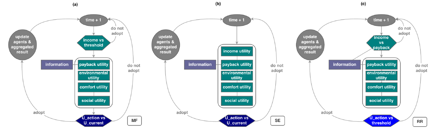
The architecture of the decision flow of MF households (Figure 1a) captures the main elements of TPB (Figure A.1, Appendix A). Our simulations run over 30-time steps, one step corresponding to a half year period. Each time step household agents in MF ABM assess their PBC implemented as a probabilistic affordability barrier (Equation 5, Table 2). It filters out households that are going to consider a PV installation decision - i.e., continue with utility estimation and information barrier check - from those who are not. Agents estimate contributions of the four decisive factors to the overall utility and weight them based on their attitudes towards these factors and social norms (Equation 6, Table 2). After estimating individual utilities of their status quo, agents continue by calculating the individual multi-attribute utility of taking an action (Equation 6), i.e., investing in PVs. Households compare this to their status quo utility to choose the highest. Since this choice of a better option is limited to the information agents posses in the current step only, this approximation of utility maximization is myopic, making agents bounded-rational (MF in Table 2). Section A.1 in Appendix A describes the MF architecture in details.
| Factors | Representation | Equation | |
| Economic | Payback period | \(u_{eco} = (t_{pv} - t_{pp}) / t_{pv}\) with \(t_{pp} = t(C_{pv} < r_{pv})\) | (1) |
| Environmental | CO\(_{2}\) emission saving | \(u_{env} = \dfrac{e^{(s_{co_2} - \overline{s_{co_2}})}}{(1 + e^{(s_{co_2} - \overline{s_{co_2}})})}\) | (2) |
| Social | Social network | \(u_{soc} = \dfrac{n_{tec}}{n_{tot}}\) | (3) |
| Comfort | Stochastic Variable | \(u_{cof}= [-1;1]\) | (4) |
| \(u\) - utility, \(eco\) - economic, \(env\) - environmental, \(soc\) - social, \(cof\) - comfort, \(t_{pv}\) - PV lifetime, \(t_{pp}\) - payback period, \(C_{pv}\) - PV costs, \(r_{pv}\) - PV revenue, \(s_{co_2}\) - CO\(_{2}\) emission saving of a particular PV, \(\overline{s_{co_2}}\) - average CO\(_{2}\) emission savings, \(n_{tec}\) - PV in neighbourhood, \(n_{tot}\) - total neighbours household | |||
We then compare MF ABM to its two alternatives inspired by the TPB-ABM of Schwarz & Ernst (2009) and the TPB-ABM of Rai & Robinson (2015), to which we further refer to as SE and RR studies. These models consider environmental, social and economic reasons for a technology investment of households whose decisions are framed according to TPB. We reproduced the SE and RR alternatives in our model code to test differences in the architecture of the TPB-ABMs. To bring the ABMs developed by SE and RR into the context of our case-study and data availability, a few adjustments were required (see Section A.2, Appendix A for details). Their corresponding approaches were implemented in our base MF ABM to create the SE and RR prototype ABMs, to which we further referred to as SE ABM and RR ABM. All the results in Section 3 are produced by the code of our ABM either under the MF, SE or RR operationalizations of TPB and parameterized using the same data from our Dutch case-study. The SE and RR ABMs reproduce architecture, factors and their representation of the TPB-based SE and RR studies. They are not reproductions of the results of the SE and RR studies.
According to the architecture of SE ABM (Figure 1b), households combine economic, environmental, social and comfort factors (Table 1) by means of a multi-attribute utility. However, the SE study introduces PBC as part of agents’ utility, instead of a two-step decision making process in MF ABM where PBC acts as a barrier between intention (utility) and behaviour (compare SE and MF in Figure 1). Each time step SE agents start directly from assessing their multi-attribute utility and employ additional weighting in the utility function: by comparing the importance of their own attitudes iatt and of PBC ipbc against the importance of prevailing social norms isoc (Equation 8-10, Table 2). Hence, SE ABM treats PBC and social norms in TPB architecturally-different compared to MF ABM.
| ABM | PBC Barrier | Utility resolution mechanism | Functional form | ||
| MF | \(th_{inc} = 1 + \dfrac{1}{e^{-n * x} + b}\) | Myopically choose the maximum | \(U_{RR,MF} = w_{eco}*u_{eco} + w_{env}*u_{env} +\) | ||
| \(th_{inc} > r\) | (5) | \(+ w_{soc} * u_{soc}+w_{cof} * u_{cof}\) | (6) | ||
| RR | \(th_{inc} > u_{eco}\) | (7) | Compare to an exogenous threshold | ||
| SE | Part of utility | Myopically choose the maximum | \(U_{SE} = (i_{att} * u_{att} + i_{pbc} * u_{pbc} ) * (1 - i_{soc})+ w_{soc} * u_{soc}\) | (8) | |
| \(u_{att} = w_{eco} * u_{eco} + w_{env} * u_{env} + w_{cof} * u_{cof}\) | (9) | ||||
| \(u_{pbc} = w_{eco} * th_{inc}\) | (10) | ||||
| \(th_{inc}\) - income threshold, \(n\) - average income, \(x\) - household income, \(r\) - random number 0-1, \(b = 6\) - shift saturation curve on x-axis, \(U\) - multi-attribute utility, \(w\) - preference/weight of each individual agent for a specific factor, \(i\) - importance, \(att\) -attitude, \(pbc\) - Perceived Behavioral Control, Definitions and equations for \(u_{eco}\), \(u_{env}\), \(u_{soc}\), \(u_{cof}\) are listed in Table 1 | |||||
As with the other two ABMs, the architecture of RR ABM is grounded in TPB (Figure 1c). RR agents start by assessing PBC implemented as an income barrier similar to MF ABM (compare RR with MF in Figure 1). The main difference between RR and MF ABMs is in the benchmark, to which this income threshold \(th_{inc}\) is compared. The MF ABM assesses PBC by comparing the income threshold \(th_{inc}\) to a stochastic value \(r\) (Equation 5, Table 2). Instead, RR ABM compares incomes to payback assessments (Equation 7, Table 2). Given that the PBC barrier is passed, RR households assess their potential utility of a PV investment decision using multi-attribute utility (Equation 6, Table 2). Their decision for or against PV is taken by comparing individual multi-attribute utilities of the PV installation to a threshold value instead of the myopic optimization in MF and SE ABMs (compare the bottom hexagons in the three TPB-ABMs in Figure 1). Consequently, the RR architecture diverges from MF ABM in how payback enters both PBC and utility assessments and in how agents form intentions by resolving utility differently. The differences between the architectures of the 3 TPB-ABMs are discussed in detail in Section A.2, Appendix A.
Different factors: Information as a new factor
Information, which consumers receive about financial aspects of a technology investment, matters (Rai et al. 2016; Yun & Lee 2015; Rai & McAndrews 2012; Kastner & Matthies 2016). Most households seeking to install PVs receive information on the financial aspects from their installers or local craftsmen (Yun & Lee 2015; Rai & McAndrews 2012; Kastner & Matthies 2016) rather than from their social network (Rai et al. 2016). If households are informed about technology by a local craftsman, his or her influence increases and the influence of the social network loses importance (Rai et al. 2016). Stakeholders’ interviews in the Dutch municipality of Dalfsen and our participatory workshop reveal that an availability or an absence of information on practical aspects of PVs installation affects individual choices (Boer 2015). Although information and information biases were important, neither was originally included in the 3 above-discussed ABMs.
In the next step, we included information as an additional factor that influences households’ decisions. Consumers consider (lack of) information on the financial aspects of the highest importance compared to information on other aspects (Rai & McAndrews 2012). Hence, information impacts individual uncertainty regarding the investment payback period (Figure 1) and therefore, is part of the economic utility (\(u_{eco}\) in Equation 1, Table 1) in MF, SE and RR ABMs. Since economic payback is part of the PBC assessment in the architecture of RR ABM (Figure A.2) the new information factor will also affect the PBC barrier (Equation 7, Table 2). Moreover, the influence of information on investment payback and final household’s decisions regarding technology could be formalized differently. Economists consider information - or time spent on acquiring this information - as additional costs, which one bears to decrease uncertainty. Traditionally in economics, these costs are monetized and added to the overall investment costs of a specific technology. In contrast, social scientists rarely appreciate a monetary representation of such an intangible factor as information. Instead, one may focus on the fact that a presence (absence) of information reduces (adds) uncertainty to an individual decision-making. Whether one presents information as monetary costs or as non-monetary uncertainty may influence the aggregated results in terms of technology diffusion. This difference in representations is just one of the possible disciplinary divides that may influence a modeller’s choice on how to implement a specific factor.
Different representations: Information from alternative disciplinary perspectives
Information as non-monetary uncertainty
Information can be represented as an (in)accuracy in individual payback calculations. According to Rai et al. (2016), 44.7% of all households considering PVs are informed on the financial aspects by their installer. Hence, in our simulations 44.7% of households estimate their payback accurately and the rest may over- or underestimate it. These remaining 55.3% of the household agents may have information biases regarding an anticipated economic payback of a PV investment (\(u_{eco}\), Equation 1, Table 1). Each time step these households are assigned an information bias regarding a possible payback of a PV investment \(r_{inf}\) drawn from a distribution \(p\) unique to each agent:
| $$r_{inf} = p(u_{eco}) \qquad$$ | (11) |
In summary, households either were informed by their installer and estimate their respective economic payback utility correctly, or they needed to search for information themselves. In the latter case, uncertainty decreases as households are better informed on the financial aspects of PV systems. The higher they estimate their economic payback utility and, consequently, their overall utility U, the higher the chances of PV adoption.
Information as monetary costs
When a household agent spends time on collecting information, associated costs can be quantified in terms of time. It is quite common - for example in transportation studies, labour market analysis or in assessing costs of illness - to express time spending in terms of monetary values. Our 3 ABMs with monetary representation of information assume that information acquisition costs are part of the initial PV investment (\(C_{pv}\), Equation 12), which together with PV revenues (\(r_{pv}\)) influences the payback period (Equation 1, Table 1).
| $$C_{pv} = c_{pv} * a + c_{inf} \qquad$$ | (12) |
The time allocated in information search could have been otherwise spent on leisure or as additional working hours, both related to monthly household incomes \(I_{mth}\). It also delays the inflow of monthly revenues \(R_{mth}\) from to-be-installed PVs. As in the transport literature, we assume that the value of this time spent constitute just a proportion \(c_{time}\) of the households' earnings, which in our case equal to the sum of monthly incomes \(I_{mth}\) and future PV revenue streams \(R_{mth}\). Waiting time costs in traffic constitutes 30% of households’ earnings (Move 2014). Following our sensitivity analysis on \(c_{time}\), we assume that the waiting time costs constitute 40% of households' earnings over the corresponding time investment.
In absence of data on the hours spent on information search, we randomly draw a value \(r_{inf}\) from a distribution unique to each agent with the mean being the economic utility estimate to capture that time investments vary across households. Hence, the monetary value of the search time investment is:
| $$c_{inf} = (I_{mth} + R_{mth}) * c_{time}* r_{inf}$$ | (13) |
Given Equations 12 and 13, the value of the economic utility \(u_{eco}\) (Equation 1) varies across the agent population based on how much time and consequently costs, they invest into the information search on financial aspects of their desired PVs. As before, we assumed that 44.7% of all households considering PVs are informed on the financial aspects by their installer. Thus, the time investment in the information search for this share of population is zero. As a result, only 55.3% of the households in our experiments spend time searching for information at their own costs, which depend on individual time investments (Equation 13). The more time they invest in the information search, the higher the initial investment costs, and therefore the lower their payback utility. Investing in the information search thus may decrease households’ chances to install PV.
Different data: Distribution of information in an agent population
Data used to parameterize \(r_{inf}\) in either of the two alternative representations of information, may impact simulation results. Rarely does a reader know the underlying distributions of data used in ABMs, since usually only averages are reported. The amount of information \(r_{inf}\) - expressed either in terms of time invested for its search or in the level of uncertainty resolved - is randomly drawn and unique for each agent (see Sections 2.9 - 2.14). We set simulation experiments to test the impact of a distribution in data behind the average value \(u_{eco}\) of \(r_{inf}\), individual to each agent.
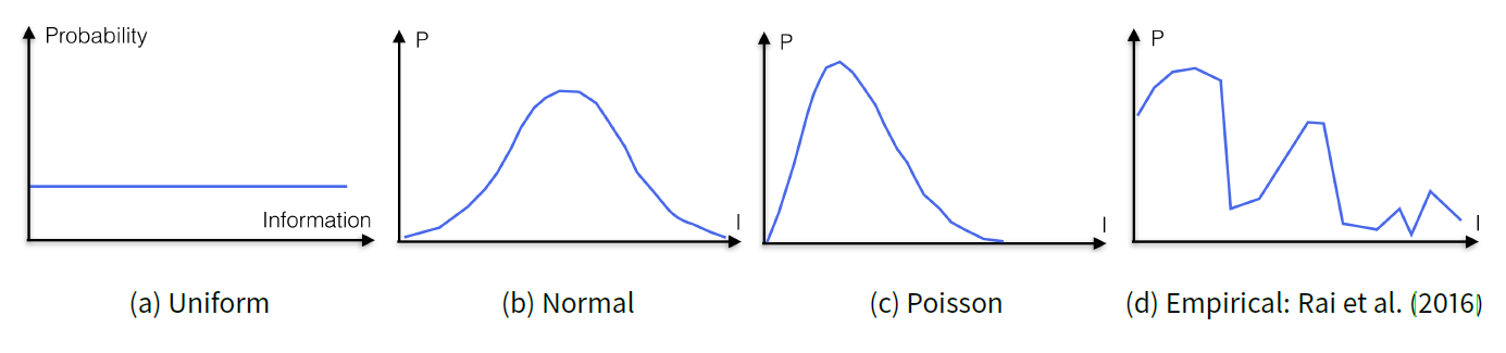
In the absence of micro-level data for the Dutch case, we used four different options to test for any qualitative differences in technology diffusion arising from the fact that unequal information was distributed among households. Rai et al. (2016) provide evidence on how much time households spend on the process of buying a PV. Considering that most of this time is spent on clarifying the financial aspects of a PV system and its performance (Rai & McAndrews 2012), we tested the performance of our three ABMs assuming that \(r_{inf}\) mirrors this empirical distribution of data. Consequently, the distribution of time spent by agents to gather information on financial aspects of PV under the monetary representation of information or the distribution of the information bias under uncertainty may look like Figure 2d. Additionally, to test the sensitivity of the results to the underlying distribution of data, we compared it with Uniform, Normal (Gaussian) and Poisson distributions (all four with identical means, Figure 2) under both representations of information.
Results
To explore the implications of various interpretations of social science theories in a formal computer code of a typical ABM, we ran a series of simulation experiments. Specifically, we ran our energy ABM using the MF, SE and RR architectures, with and without information as an additional factor (see Sections 2.7-2.14). When present, the information factor was implemented either as monetary costs or as non-monetary uncertainty and was tested under each of the four random distributions of \(r_{inf}\) (see Sections 2.9-2.16). In addition, an extensive sensitivity analysis was performed, including such parameters as thresholds on income and PBC in MF and RR ABMs and the initial value of the importance of attitude in SE ABM. We ran each combination of settings 50 times, resulting in 1950 simulation runs across all model versions. We reported the simulation results in terms of technology diffusion curves to indicate the differences in the overall spread of PV adoption and in its temporal pattern. Each figure illustrates the mean diffusion curve across the 50 repeated runs under the same settings; the standard deviation is small (Table 3). In addition, Table 3 presents the resulting regional green energy production, estimated as
| $$E_{tot} = e_{max}* t_{sun} * p * a \qquad$$ | (14) |
| $$S_{co2} = E_{tot} * \overline{s_{c02}}\qquad$$ | (15) |
| $$S_{mon} = r_{tot} - C_{pv}\qquad$$ | (16) |
Different architecture
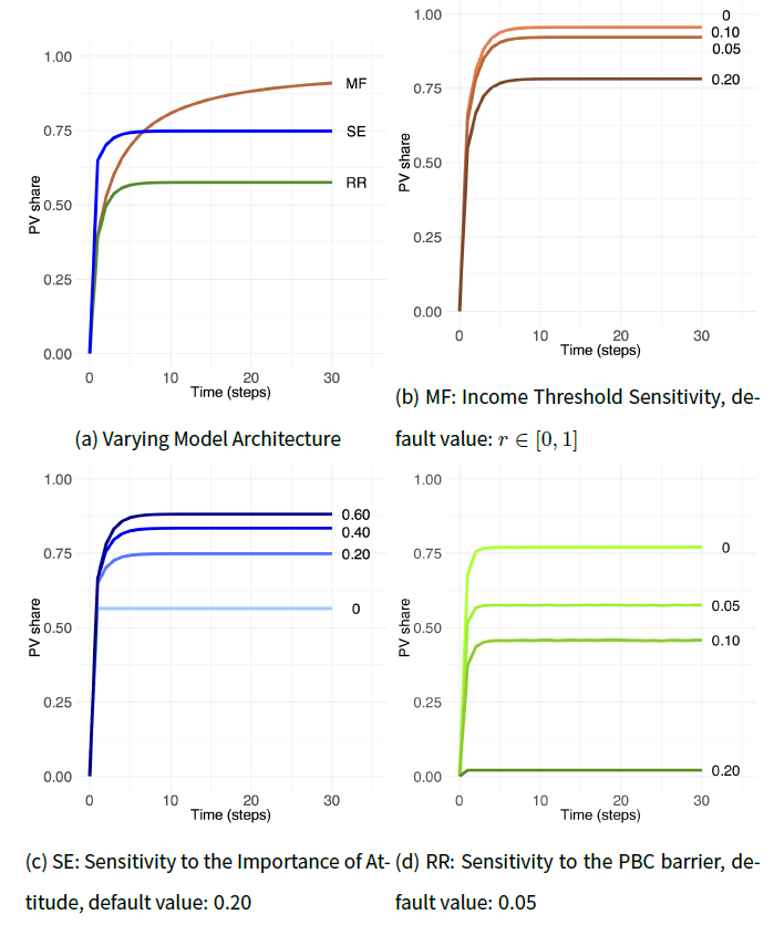
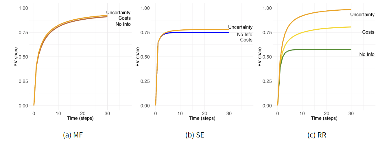
Figure 3a compares PV diffusion rates under various implementations of the same social science theory - TPB - in MF, SE and RR ABMs. The differences in the model architecture are evident: depending on a modeller’s choice when interpreting subtle qualitative psychological concepts, the resulting technology diffusion rates vary significantly from 58% in RR, to 75% in SE and 91% in the MF models, ceteris paribus. This means 16%-33% less renewable energy produced in SE and RR ABMs compared to MF, with proportional consequences for emissions and monetary savings. Notably, the differences in the models’ architectures interact in a complex way. While MF and SE ABMs share the same assumption on the utility resolution mechanism (Table 2), the MF and SE diffusion curves are qualitatively different (Figure 3a). The same is true for the MF and RR diffusion curves (Figure 3a) despite the fact that these models share the same assumption of the PBC assessment preceding the utility estimation (see MF and RR in Figure 1), which has the same functional form (Table 2). The three PV diffusion curves differ, with SE and RR architectures producing qualitatively similar shapes although there are different mechanisms leading to it. The speed of diffusion also varies, as indicated by the saturation points in Figure 3a. The results from SE and RR ABMs indicate that there were almost no more adopters observed starting from the period 4 and 5 respectively. Yet, the spread of PVs continues in MF ABM until time step 28, overshooting the final diffusion rates at the end of the observed period by 18% and 37% compared to SE and RR ABMs respectively.
Figures 3b-3d and Appendix B present a sensitivity analysis of the three base models (Figure 3a) to their crucial exogenous architectural parameters. Namely, the benchmark r (Equation 5) to compare the income threshold in MF ABM, the importance of attitude \(i_{att}\) (Equation 8) in SE ABM, and the PBC barrier threshold \(th_{inc}\) (Equation 7) in RR ABM probably impacted the results. The RR architecture was the most sensitive of the three models with results varying by almost 97% between the base value of 0.05 and 0.1-0.2 settings (Figure 3d). The difference from the default values in MF and SE ABMs was a maximum of 14% and 25% respectively (Figure 3b and 3c).
| Architecture | Representation of information | Data | Diffusion rate [0,1] | Energy production [106 GWh/yr] | CO\(_{2}\) savings [ktonne/yr] | Monetary savings [106 EUR] |
| MF | Baseline | — | 0.910(0.004) | 316(1.1) | 3533.8(12.3) | 251(0.9) |
| Uncertainty | uniform | 0.923(0.003) | 320(1.0) | 3578.5(11.3) | 254(0.8) | |
| normal | 0.914(0.003) | 317(1.0) | 3544.8(11.2) | 252(0.8) | ||
| poisson | 0.912(0.003) | 316(1.1) | 3539.1(12.3) | 252(0.9) | ||
| empirical | 0.907(0.004) | 315(1.2) | 3524.0(13.0) | 251(0.9) | ||
| Monetary | uniform | 0.910(0.003) | 316(0.9) | 3535.2(9.9) | 251(0.7) | |
| normal | 0.910(0.004) | 315(1.2) | 3533.5(13.2) | 251(0.9) | ||
| poisson | 0.909(0.003) | 315(0.8) | 3530.9(9.4) | 251(0.7) | ||
| empirical | 0.910(0.003) | 316(1.0) | 3533.2(11.2) | 251(0.8) | ||
| SE | Baseline | — | 0.748(0.004) | 253(1.6) | 2836.3(17.5) | 202(1.2) |
| Uncertainty | uniform | 0.781(0.004) | 265(1.6) | 2967.7(17.6) | 211(1.3) | |
| normal | 0.762(0.004) | 258(1.6) | 2890.5(18.0) | 206(1.3) | ||
| poisson | 0.760(0.005) | 257(1.9) | 2883.7(21.8) | 205(1.6) | ||
| empirical | 0.774(0.004) | 263(1.6) | 2939.8(17.7) | 209(1.3) | ||
| Monetary | uniform | 0.749(0.005) | 253(1.7) | 2838.3(19.3) | 202(1.4) | |
| normal | 0.748(0.005) | 253(1.8) | 2835.7(20.3) | 202(1.5) | ||
| poisson | 0.749(0.005) | 254(1.5) | 2839.7(16.26) | 202(1.4) | ||
| empirical | 0.748(0.005) | 253(1.7) | 2835.3(19.75) | 202(1.4) | ||
| RR | Baseline | — | 0.576(0.003) | 226(0.8) | 2534.5(9.4) | 180(0.7) |
| Uncertainty | uniform | 0.984(0.002) | 337(0.3) | 3777.8(3.7) | 269(0.3) | |
| normal | 0.898(0.003) | 318(0.8) | 3566.6(9.4) | 254(0.7) | ||
| poisson | 0.820(0.002) | 300(0.6) | 3361.6(6.6) | 239(0.5) | ||
| empirical | 0.982(0.002) | 336(0.5) | 3766.7(5.2) | 268(0.4) | ||
| Monetary | uniform | 0.810(0.005) | 297(1.8) | 3321.7(20.3) | 236(1.5) | |
| normal | 0.696(0.064) | 259(19.5) | 2896.5(218.0) | 206(15.5) | ||
| poisson | 0.697(0.064) | 259(19.4) | 2899.2(216.9) | 206(15.4) | ||
| empirical | 0.602(0.017) | 232(4.2) | 2602.9(47.5) | 185(3.4) | ||
| 50 random seed runs per configuration | ||||||
Different factors
Figure 3a illustrates the aggregated regional PV diffusion trends in MF, SE and RR ABMs assuming that economic, environmental, social and comfort factors influence individual decisions of households. Here we tested how adding information as a decisive factor impacted the emergent PV diffusion rates in each version of the TPB-ABM architecture (Figure 4). In this set of simulation experiments, the lack of information comes as agents’ uncertainty regarding the financial aspects. The key variable \(r_{inf}\) was parameterized using secondary data on time spent to clarify financial aspects of a PV system and its performance (Rai & McAndrews 2012). Instead of assuming that households were perfectly informed of PVs performance and their financial consequences, we assumed that a population of agents was heterogeneous in the level of information they possess. Consequently, some household agents may have over-or underestimated the economic payback.
As in the base case (Figure 3a) the curve shapes and final rates of adoption varied across the three architectures (Figure 4). Interestingly, an inclusion of information as an additional factor in an individual decision process made little difference to the resulting regional diffusion rates in MF ABM. According to this model, a population of agents with objective information is likely to install as many PVs as the population that partially lacks information and may over- or underestimate the economic utility of undertaking the action. In the presence of information biases, MF ABM demonstrated a slightly lower PV share only initially (time steps 5-15). This difference disappeared when both curves - with and without information bias - approached a steady state, implying that full information provision barely impacts renewable energy production, CO\(_{2}\) savings and cumulative financial benefits for households in the region (MF-Baseline vs. MF-Uncertainty-Empirical, Table 3). Similarly, the PV diffusion curve was initially below the baseline when information bias was included in SE ABM (Figure 4b) but gradually overtook the baseline curve around time step 7. The steady state PV share in the presence of information bias was 77% compared to 75% in the base SE ABM. Hence, when part of the SE agents over- and underestimated economic utility, there was 3.5% improvements in the regional sustainable energy production.
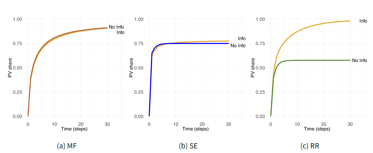
The inclusion of information as an additional factor mattered most for RR ABM (Figure 4c). In contrast to MF and SE ABMs, information influenced more than economic utility \(u_{eco}\) alone. Given the architecture of RR ABM information was now also part of the PBC assessment (Figures 1 and A.2). When households agents over- and underestimated their payback, in turn influencing the PBC barrier, the regional impact on PVs diffusion was significant. Only 58% of the population invested in PVs when they were fully informed compared to 98% when households had an information bias (Table 3). Hence, incorrect information in these model settings on average led to overoptimistic assessments of individual benefits and resulted in 71% more regional renewable energy and \(CO_{2}\) savings. In the model this is likely to be sensitive to PV costs and whether they fall over time as more adoption occurs, testing for which is outside the scope of the current article. Apart from the steady state, there was a difference in the diffusion process in RR ABM. With information bias, the increase in PV investments occurs slower, leading to the steady state being reached in step 30 instead of 10 in the baseline RR ABM. The shape of the RR-Information curve is similar to that of MF (Figure 4a). By introducing a stochastic element \(r_{inf}\) to the RR PBC barrier, we make it resemble the MF probabilistic income barrier. Hence, two different factors may have a similar effect on model behaviour under given different architectures.
The purpose of this paper was not to test which model version is correct. Rather we aim to quantitatively explore the implications in the differences of interpreting qualitative concepts in the formal code of a simulation model. If the three models were to include information about PVs performance and their financial consequences as a new factor that varies among household agents, they would arrive at different conclusions. The RR ABM indicated that a fully informed population of households invests less compared to the one that either underestimates or overestimates an economic payback. When used to explore information policy impacts - such as running information campaigns or creating incentives to make information on PV specification and costs more accessible to public - the RR architecture would imply that communicating full objective information on financial consequences has adverse effects in terms of reduced PV diffusion (given fixed costs of technology). Instead, the outcomes of MF and SE ABMs suggested that an information policy would not have a significant effect. Given the crucial importance of these implications, more research is needed on the validation of the assumptions about behavioural drivers and their integration in formal models (ABMs or others).
Different representations
To further explore how information of PV specifications and costs influenced households decisions, we compared results of our ABMs with the representation of information as uncertainty vs. as monetary costs (see Sections 3.8-3.16). Figure 5 illustrates dynamics of PV diffusion rates among households in the region under the two alternative representations of information in MF, SE and RR ABMs. For both alternatives we ran a sensitivity analysis to understand how emergent diffusion rates change with different underlying values and distribution of the key parameter \(r_{inf}\) (Table 3), to be discussed further in Sections 3.12-3.16. Figure 5 shows only the results of the three ABMs with \(r_{inf}\) parameterized using the Uniform distribution as the one that shows the most important differences between the two representations of the information factor in the models’ code.
Figures 5a and 5b revealed no differences in the regional diffusion of PVs between the base MF and SE ABMs with no information and when households incur additional costs to search for information on PV specifications. Information as costs had a small impact on the economic payback utility. Since the latter is also weighted by each individual household agent against other important factors such as comfort, environmental and social aspects, information as costs play an insignificant role in the overall decision on whether to install PVs in these two ABM architectures. The drastic difference occurs in RR ABM where information as costs enters both the economic utility and the PBC barrier. RR agents start investing time in searching for information on the financial costs of a PV investment given the size of their house. Even if they do it at their own costs, their payback estimates allow them to pass the PBC barrier. Compared to the baseline with no information, the compound effect of these individual dynamics results in 41% higher overall diffusion rates of technology and 49% more renewable energy produced at the regional scale (Table 3).
A representation of ’information as uncertainty’ showed a difference compared to ’information as costs’ or ’no information base case’ in all 3 ABMs[1]. Figure 5 illustrates that emerging diffusion rates go 1.4% and 4.4% up when information represented as uncertainty enters agents’ decision-making in MF and SE ABMs correspondingly, given that with \(r_{inf}\) follows the Uniform distribution. In RR ABM, the presence of information as uncertainty triggered a 71% increase in PV adoption and made a difference in how quickly the steady state PV share is reached. When uncertainty in financial information enters households decision making, it took 5 times longer to reach saturation point (time step 29 instead of 5 in the absence of the information factor, Figure 5c.
Hence, even given a single theory explaining individual behaviour there could be variations in the way specific factors are represented in ABMs, potentially leading to different conclusions. Our example with two options to represent the influence of information as a decisive factor indicates 1.4%, 4.1% or 18% difference in resulting PV shares between runs with information as uncertainty vs. information as costs in MF, SE and RR ABMs (Table 3, Uniform distribution).
Different data
Lastly, we ran analyses to explore how PV diffusion curves change with a distribution of \(r_{inf}\)(Figure 2), with each agent keeping their individual mean value. When information was represented as costs, most of the runs across our 3 ABMs and 4 distributions show no qualitative difference compared to ’no information’ case, except RR ABM. Thus, in addition to the latter case, we further discuss only the variability in results of the three ABMs with information represented as uncertainty under the four distributions of \(r_{inf}\) (Figure 6).
A population of households with different information endowments representing uncertainty over their PVs’ payback in MF ABM shows robust patterns (Figure 6a) as does a society of agents in SE ABM (Figure 6b). In the case of MF ABM, the diffusion rate of PV with information biases parameterized using Poisson, Uniform and Normal distributions and multi-modal distribution that follows the patterns from the secondary data source, nearly match the base case with no information (black horizontal line in Figure 6a). The largest difference is in the case of uniform distribution. The results depict a slight increase in the PV investments carried out by 92% of regional population instead of 91%, when information is absent, increasing green energy production, CO\(_{2}\) savings and financial benefits of households by 1.2% - 1.3% (Table 3).
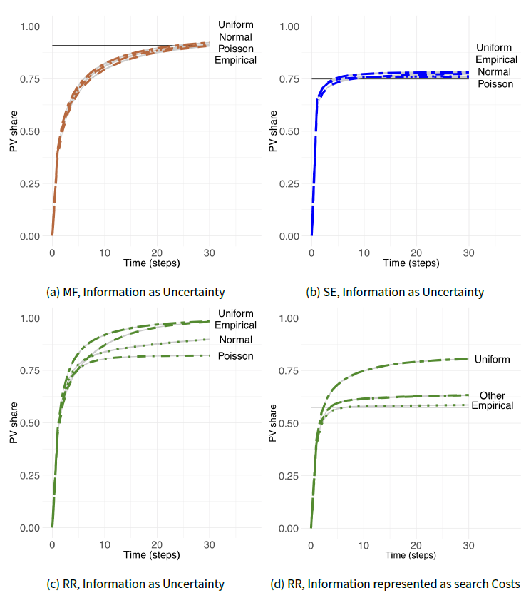
The interactions in the population of SE ABM parameterized with Uniform, Normal and Empirical distributions of \(r_{inf}\) led to diffusion curves that cluster above the baseline value without any information biases (Figure 6b), meaning that more agents over- than underestimate their payback. The maximum overestimation compared to the ’no information’ baseline (+4.4% difference) occured in the population of SE agents with information biases distributed following the Uniform distribution.
The case of the RR architecture, where information impacted both the economic utility and the PBC assessment, illustrates the most pronounced effect. The compound effect of information affecting these two factors influenced the results under both representations of information: as uncertainty and as costs. As Figure 6c illustrates, more household agents were prepared to invest in PVs compared to the baseline, regardless of the distribution behind individual uncertainty on financial aspects. The PV diffusion is increased by 71%, 71%, 56% and 42% when agents’ information biases follow Uniform, Empirical, Normal and Poisson distributions, leading to 33%-49% difference in green energy production, CO\(_{2}\) savings and financial benefits of households (Table 3). When costs of information search are monetized and enter households PV investment decisions, the RR population endowed with Uniform \(r_{inf}\) was 41% more willing to install PVs (Figure 6d). When costs of information follow the multi-modal empirical distribution, the diffusion curve nearly follows the baseline. Overall, RR ABM shows a total variation of steady state PV share of around 64% across the different information representation and distributions, which was higher than for either in the SE or the MF case.
Notably, all the curves in Figure 6 were from the same set of average values per agent of \(r_{inf}\). The shape of the distribution - Normal, Uniform, skewed Poisson or multi-modal empirical - determined the initial households endowments of this stochastic information factor, which were further impacted through social interactions, individual income levels and other decision variables. Hence, there was no clear pattern on whether a particular distribution affects diffusion rates in a predefined direction: the relationships are non-linear and are influenced by both the architecture of the models and the representation of information as an additional factor. Consequently, it is vital to consider them in combination when assessing behaviour of a particular model.
Conclusion
As agent-based modelling gains popularity, the demand for transparency in underlying modelling assumptions grows. Behavioural rules guiding agents’ decisions, learning, interactions and possible changes in these should rely on solid theoretical and empirical grounds. The field has matured enough to reach the point that we need to go beyond just reporting what social theory we base these rules upon and listing average values of data used for parameterization. Many theories operate with various abstract constructs such as attitudes, perceptions, norms or intentions. These concepts are rather subjective and remain open for interpretation when operationalizing them in formal model code. As a number of ABMs based on the same theory grows, it becomes increasingly important to compare how the same theory is implemented in various models. This paper aims to shed light on the consequences of variations in formalizations of a social science theory on the simulation outcomes of ABMs of the same class - models grounded in the same theory and designed to address the same research problem. Four types of differences are considered: in model architecture concerning specific equations and their sequence, in factors affecting agents’ decisions, in the representation of these factors potentially from different disciplinary perspectives, and finally in the underlying distribution of data used in a model. We illustrated emergent outcomes of these differences using the example of an agent-based simulation model, which is developed to study regional impacts of household solar panel investment decisions, and applying the Theory of Planned Behaviour as one of the most common social science theories used to define agents’ behavioural rules.
With respect to architecture - types and sequence of equations and if/else rules in which different factors influencing decisions are assembled - we designed the ABM inspired by TPB-ABMs from the literature. The simulation results under 3 different TPB implementations varied both quantitatively, in terms of the maximum share of population investing in PVs (91%, 75% and 58% in MF, SE and RR ABMs correspondingly), and qualitatively, in terms of shapes of diffusion curves and the timing of the saturation point (time step 28 in MF vs. 5 and 7 in SE and RR). Consequently, there was 18% (according to SE TPB-ABM) and 37% (RR TPB-ABM) less green energy produced, fewer CO\(_{2}\) emissions prevented and less cumulative financial benefits for households achieved in the region compared to the MF ABM. Importantly, slight differences in the interpretation of a qualitative social science theory, which lays the foundations of behavioural rules of individual agents in the code of a formal model, get amplified when applied to thousands of agents and lead to significant deviations in the emergent outcomes.
Motivated by the empirical literature and the feedback from our stakeholder workshop, we introduced information on PV installation as a decision factor in addition to economic, environmental, comfort and social aspects important to households’ agents. While one may expect a deviation in simulation results with an addition of a new factor, we found that the effects depend on the model’s architecture and was sensitive to a particular representation of the information factor. We scrutinize our models by introducing two means of representing information on PVs: as uncertainty regarding the payback and as monetary costs of searching for information. Indeed, we contrasted a formalization of quality of information represented as inaccuracy in PV payback assessments, with quantity of information, measured in cost of time spent to reduce uncertainty. The implementation of the inaccuracy of information caused changes in the steady state PV share for all 3 ABM architectures. The introduction of information costs however, made no significant difference for MF and SE ABMs, while for RR ABM the system behaviour depended on the distribution of information among individual households. Therefore lastly, we ran three TPB-ABMs varying in architecture, each with two alternative representations of information where a crucial stochastic parameter is initiated following four different data distributions with individual agents’ same average value. Our results indicate qualitative and quantitative differences in the emergent outcomes such as technology diffusion rates with changes across model variations ranging from 1% to 71% and a steady state being reached on step 5 vs not being reached even after 30 periods. It impacted the simulated values of produced renewable electricity and saved CO\(_{2}\) emissions, which vary between 226e6 - 337e6 GWh/yr and 2534.5 - 3777.8 ktonne/yr correspondingly and potentially lead to different conclusions and policy implications from the simulations. We found no clear pattern on whether a Uniform, Normal, skewed Poisson or multi-model Empirical distribution affects diffusion rates in a predefined direction. The relationships wee non-linear and were influenced by both the architecture of the models and the way one represents information. Hence, it is vital to consider the four types of differences in combination when assessing behaviour of a particular model.
Our work has several methodological implications.
- Transparency on implementation and systematic tests: From a modelling perspective there could be different ways to formalize qualitative social science concepts in a formal model (Polhill & Gotts 2017; Köhler et al. 2018) The way such intangible notions as social norms, attitudes, perceived control and alike are implemented in a model, influences results both qualitatively and quantitatively. The sensitivity of results to the four types of tested differences indicate that emergent PV diffusion rates vary between 0.98 and 0.576. Hence, the transparency and reliability of any modelling results depend on whether the consequences of variations in the interpretations of the same social science theory in ABMs of the same class are well understood. Other studies performing a systematic analysis for the four types of differences - architecture, factors, representations and data - are desirable. Future research could focus on revealing the status of using other social science theories (beyond TPB) in bottom-up computational models.
- Modellers & behavioural scholars: Despite the fact that TPB is often used by modellers, some interpretations of its concepts remain questionable and would ideally require a serious consultation with psychology scholars to resolve ambiguities. Our modelling exercise has revealed three aspects where the theoretical interpretation of the TPB use in the modelling literature should be challenged. Firstly, according to Ajzen (1991), PBC is a combination of self-efficacy and controllability. Yet, to our knowledge the PBC assessment comes only as a test for controllability in ABMs represented by economic (in most ABMs) and sometimes physical constraints (as in the original Rai & Robinson (2015) study). The fact that it omits other possible aspects - such as perception of individual efficacy and psychological stimuli to undertake an action - is debatable. Secondly, while TPB differentiates between the individual intention and the actual action (Figure A.1) the step between them is insufficiently represented in current ABM literature. The utility function assesses agents’ intentions in MF and RR ABMs and PBC should mediate between intentions and actions. Yet, it is done indirectly: to minimize the computational time, we reverse the order by assessing agents’ PBC first and then going through a more computationally intensive multi-attribute utility estimation with a smaller share of population. SE ABM has PBC within the utility function undermining the difference between a one-step and a two-step decision making process. Moreover, in all three ABM implementations we tested here, PBC is approximated to agents’ actual behavioural control instead of perceived behavioural control (Ajzen 1991). The difference between the actual and the perceived assessments could be modelled as a delay function of the actual calculated value as in System Dynamics literature (Sterman 2000) or by explicitly representing self-efficacy in the PBC assessment. The discussion on how and where the PBC barrier should appropriately be set from a conceptual perspective is an important point that could be resolved in collaboration with psychologists. Thirdly, conceptually TPB distinguishes between attitudes towards behaviour and subjective norms Figure A.1. The modelling literature merges both within the multi-attribute utility function (Tables 1 and 2). The architecture of MF and RR ABMs assumes that subjective norm is one of the 4 decision factors, which are weighted against each other with weights equal to individual attitudes towards all four. SE ABM treats attitudes towards a particular technology apart from technology-specific weights for main decision factors. The decision to implement subjective norms and attitudes in a particular way is not explicitly reasoned by modelers in the published literature and is not contested by behavioural scholars who study these processes empirically. In summary, the conceptual interpretation and validity of these modelling assumptions from the psychological point of view remains unclear. Moreover, modellers get locked into a particular theory that has been used for a class of decision-making problems before, overlooking the state-of-the-art advances in psychological research. The dialogue between the two worlds - behavioural sciences and simulation modelers - could lead to a better understanding of qualitative concepts, their more elegant implementation in formal models and potentially to improvements in behavioural theories. The Consumat approach (Jager et al. 2000) is a good example of a collaboration between modellers and social scientists. Not only does it diminish ambiguity in interpretations of behavioural concepts in ABMs, but also sharpens the theory by aligning its qualitative concepts with empirical data on behaviour through joint development of questionnaires grounded in theory and designed to fit ABMs (van Duinen et al. 2016).
- Micro-level data on behaviour: We will not repeat here the acute need for empirical data to parameterize and validate ABMs (Robinson et al. 2007; Windrum et al. 2007; Smajgl et al. 2011). Rather, we focus on the use of empirical data grounded in a behavioural theory to specify decision and interaction rules of agents. The ambiguity in modellers’ interpretation of vague theoretical concepts, as the TPB-ABM issues discussed in the point above, might be potentially resolved by a thorough analysis of micro-data to actually test whether all the theoretical components are significant and how they are connected. In other words, the empirical validity of a theory in a particular context should precede the modelling stage. It might seem obvious, yet the problem is in the inherit feedback between behavioural data collection and validation of a theory, in which a particular questionnaire or behavioural experiments are grounded. Namely, we collect only the information that we ask for. Thus, if our data collection omits a measurable proxy of a specific intangible concept, we cannot test a relationship that may appear obvious during the modelling stage. Hence, a recursive process is needed, where the design of behavioural data collection grounded in a theory should go hand-in-hand with the development of a stylized ABM grounded in the same theory. The latter calls for a sharper questionnaire formulation to be able to derive proxies for qualitative concepts, and often provides insights on unexpected system behaviour, demanding additional questions to test relationships earlier unforeseen by this theory. Besides, data on individual decision making is essential when extending one theory with the insights from another, as in our ’information factor’ example. Our representation of information deals either with its quantity or quality, stemming from different theoretical stands and leading to different kinds of conclusions from the simulations. Future research should focus on how (lack of) information impacts individual decisions, for example on energy technology adoption, and how trust and search time and/or costs influence individual behaviour. Studying this empirically on large datasets will help differentiating between competing theories.
- Standardization and modular approach for alternatives: Theories of human decision-making in various contexts provide an essential ground for understanding cause-effect links between stimuli or barriers and individual actions, and feedbacks between individual decisions and social norms or policies. As such they serve as micro foundations for designing agents’ behavioural rules necessary for any solid academic use of the ABM method. Moreover, results of theory-grounded ABMs can be directly compared to conventional analysis (empirical, statistical or analytic) driven by the same theory, which serves as a natural benchmark for comparison with advanced agent-based simulations. Yet, to continue using social science theories in ABMs the modelling community needs to systematize the way, in which we implement them to gain a better control on assumptions that qualitatively influence models’ results. Ideally, one would like to have an open-access open-source library of standardized modules with implementation of different social science theories accommodating points 1-3 above. Storing and sharing of reusable modules rather than entire models, often too complex and rigid to be recyclable, has multiple advantages (Bell et al. 2015). The modelling community may polish the implementation of most commonly used behavioural theories and potentially agree upon a standard way to code them. Having such a library of modules would significantly boost the scientific and practical value of models, help reusing and constantly improving them. Naturally, the theory implementation in a code as differentiated along the 4 dimensions (architecture, factors, representation and data) may depend on a case-study context. Therefore, the library of decision-making theories modules could still - and even most likely will - contain a number of alternative peer-reviewed modules implementing a behavioural theory in a computer code. Even though alternative implementations may exist, exposing modules’ architecture to scrutiny could stimulate the modelling community convergence on the issue. The modular approach to code sharing is a prominent direction in modelling (Voinov & Shugart 2013; G. & Schulze 2016) and the open-source movement is on a rise (Janssen 2017). It makes it a perfect momentum to expose and discuss openly the assumptions behind implementing a particular theory in an ABM. Importantly, given the open-source nature of the code sharing facilities such as CoMSES Network, these modules are subject to the natural evolutionary process as new evidence on their performance is appearing, either validated against data or tested with a critical eye of behavioural scholars.
The identification of four different sources of disagreement in the computational social science models does not imply that one needs to abandon the method all together. These hidden differences in subtle modelling nuances are common among all types of modelling, including land use models (Alexander et al. 2017), macro-economic computable general equilibrium models (Koks et al. 2016; West 1995) and integrated assessment models (Greenstone et al. 2013). Indeed, agent-based modelling has a clear advantage for resolving this methodological challenge. Other modelling approaches suffer from having weak theoretical grounds (Stern 2016; Pindyck 2013; Meyfroidt 2016), that at times hinder understanding of data patterns. ABMs have a unique position to connect observed decision-making, including participatory settings (Barreteau 2003; Voinov & Bousquet 2010; Elsawah et al. 2015), and a variety of theories developed by behavioural scholars. Inherit to its nature, the agent-based method links individual behavioural data and decision rules to observed aggregated phenomena, serving as a vehicle to support social sciences in addressing the classical micro-macro-aggregation problem (Coleman 1990; Forni & Lippi 1997; Kirman 1992) and making it a win-win collaboration. Future work along the four directions outlined above will assure solid grounds for theoretical micro-foundations of ABMs, aligned with data and state-of-the-art achievements in behavioural sciences. Addressing this challenge makes agent-based modelling a mature scientific method, assuring a higher credibility, especially when providing a policy advice.
Notes
- Results also depend on the assumption about the distributions of the micro-level data on the \(r_{inf}\) value, as discussed in details in Sections 3.12-3.16.
- The value of importance parameter is not provided in the paper Schwarz (2009).
- It is worth noticing that, while the MF and RR ABMs do include PBC to mediate between intention and action, they do it indirectly. Specifically, to minimize the computational time, it is done in the reversed order before assessing the intention to filter out the agent population that will not go through a more computationally intensive multi-attribute utility estimation. It makes no difference for the results though.
Appendix
Alternative implementations of Theory of Planned Behaviour in ABMs
A.1 The base model: Theoretical and empirical background
Theory of Planned Behaviour
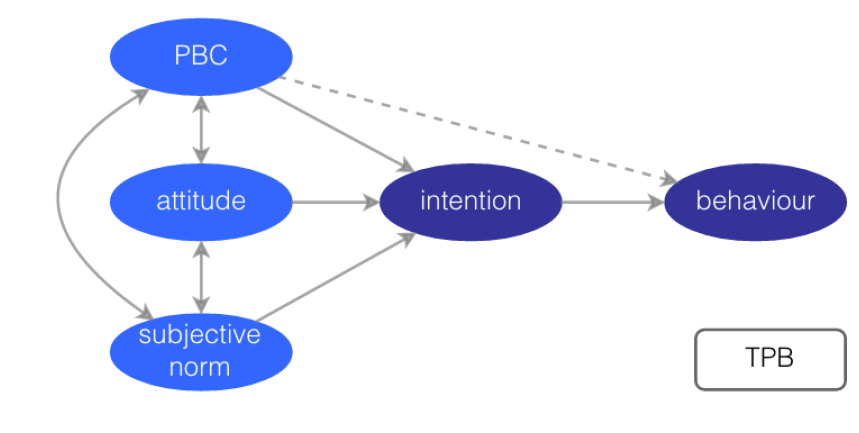
TPB was introduced by (Ajzen 1991) who suggests that human behaviour is driven by behavioural beliefs (attitudes), normative beliefs (subjective norms currently prevailing, peer pressure as perceived by an individual) and beliefs about facilitating or impeding factors (perceived behavioural control). These three trigger a formation of an intention to act (Figure A.1). Perceived behavioural control (PBC) serves as a proxy for an actual behavioural control, and may represent a barrier between intentions and actual choices (Yun & Lee 2015).
The TPB is extensively used in ABMs. TPB-ABM are used to study technology diffusion among households (Schwarz et al. 2016; Schwarz & Ernst 2009; Robinson & Rai 2015; Gamal Aboelmaged 2010), migration decisions (Klabunde & Willekens 2016; Kniveton et al. 2012, 2011), farmers’ decision making (Kaufmann et al. 2009), healthy lifestyle choices (Richetin et al. 2010), waste recycling (Ceschi et al. 2015), adoption of food safety measures (Verwaart & Valeeva 2011), urban development (Silva & Wu 2014) and segregation decisions (Wang & Hu 2012), traffic behaviour (Roberts & Lee 2012; Yu & Gou 2014) and ethical problem solving (Robbins & Wallace 2007). This makes of TPB a good case of a social theory for the purpose of this article.
An agent-based model to study energy technology diffusion in the Netherlands
The ABM, which we take as a basis for testing the four types of differences - in architecture, factors, representations and data - is developed to study the diffusion of renewable energy among households (Tariku 2014; Muelder 2016). We refer to this base version as to the MF ABM (after the authors). The MF ABM is designed to study the aggregated outcomes of individual household decisions regarding PV installation in a municipality of Dalfsen, which is one of the pioneering green municipalities in the Netherlands. There are 5800 agents that represent houseowners of various income classes spread over the spatial landscape. The model is coded using NetLogo (Wilensky & Evanston 1999); the model code is available online, under this link.
We use GIS data, data on income distribution and accommodation sizes provided by the Dalfsen municipality (Boer 2015). In addition, we elicited factors, which play a role in solar panel (PV) installation decisions of people, and their relative importance (weights) during a participatory workshop in late 2015 (Flacke & de Boer 2016), followed by a small focus group questionnaire in 2016 (Moghayer et al. 2016; Tariku 2014). Four factors appeared important for people when considering PVs: financial considerations, environmental impact, psychological comfort (displeasure or esteem), and familiarity or experience with PVs within their social network. In addition, participants of the workshop indicated that a lack of practical information (differences between types of PVs, their effectiveness and costs, reliable providers) served as a barrier. Most of these factors are discussed in the empirical literature (Yun & Lee 2015; Rai & McAndrews 2012; Kastner & Matthies 2016; Rai et al. 2016) and all factors except ’information’ have been studied earlier in the ABM literature (Robinson & Rai 2015; Palmer et al. 2015; Rai & Robinson 2015; Schwarz & Ernst 2009; Bravo et al. 2013).
Representation: Following the participatory workshop discussions, we characterize households’ agents decision-making in the MF ABM based on the four factors using specific measures (Table 1). The economic factor (\(u_{eco}\)) is represented as a payback period of a PV (\(t_{pp}\)) relative to its lifetime (\(t_{pv}\)), Equation 1 in Table 1). The environmental impact factor (\(u_{env}\)) is represented by the total CO\(_{2}\) emission savings through the lifetime of to-be-installed PVs. This factor depends on the specific CO\(_{2}\) emission savings for a household, the technology in question (\(s_{co_{2}}\)), the average emission saving (\(\overline{s_{co_{2}}}\)) for that technology (Equation 2, Table 1), and follows an S-shaped function. The CO\(_{2}\) emission savings are approximated using the reduction of CO\(_{2}\) emissions of each household's PV cell in comparison to fossil energy sources over the course of the PV lifetime in tonnes. The social factor (\(u_{soc}\)) is based on the share of technology users (\(n_{tec}\)) in a households social network (\(n_{tot}\)) (Equation 3, Table 1). In the MF ABM each household agent is connected to three household of the same income class, making the "social grouping" based on shared socio-economic background (Sociovision 2004, 2007; Mollenhorst 2015). Lastly, psychological comfort (\(u_{cof}\)) represents either the esteem that individuals experience due to owning PVs or the individual dis-pleasure due to a spoiled view. This factor is represented as a stochastic variable [-1;1], assuring that our agent population has a variety of positive and negative attitudes towards PV (Equation 4, Table 1).
Architecture: The decision flow (Figure 1a) captures the main elements of the TPB. Each time step household agents in the MF ABM assess their PBC implemented as a probabilistic affordability barrier. It filters out households that are going to consider a PV installation decision - i.e. continue with utility estimation and information barrier check - from those who are not. Instead of having a cut off income criteria, we assume that all house-holds have a chance to consider this decision (Equation 5, Table 2), but household agents with a higher income are more likely to do it (Ameli & Brandt 2015; Ramos et al. 2015). In Equation 5 each household’s income (\(x\)) is normalized by the average household income (\(n\)), and the distribution of an income threshold (\(th_{inc}\)) over all household follows a saturation curve with a value which increases with income.
Household agents continue with explicit assessment of their PV decisions after the PBC consideration. Namely, agents estimate contributions of the four decisive factors to the overall utility and weight them based on their attitudes towards these factors and social norms (Equation 6, Table 2). After estimating individual utilities of their status quo, agents continue with calculating the individual multi-attribute utility of taking an action (Equation 6), i.e. investing in PVs. Households agents compare it to their status quo utility and choose the highest of the two. Since households choose the best option in accordance with their utility given a horizon of the current time step only, their optimizing behaviour is bounded to the timing of their decisions. Given this imperfect information, agents utility maximization is not global making them myopic making agents boundedly-rational (Table 2). All global variables of interest such as diffusion rate of the technology and social norms are regularly updated (Figure 1a).
A.2 Different architectures: Theory of Planned Behavior in ABMs
As any other social science theory, TPB operates with theoretical constructs such as beliefs, norms or PBC, that creates deviations in how they are operationalized in an ABM. Let us compare two cases: a TPB-ABM of Schwarz & Ernst (2009 ) and a TPB-ABM of Rai & Robinson (2015), to which we further refer as SE and RR studies correspondingly. Both models consider environmental, social and economic reasons for a technology investment, and are based on TPB and multi-attribute utility theory. We reproduce SE and RR alternatives in our base MF model to be able to test differences in the architecture of TPB-ABMs. To bring the ABMs developed by SE and RR into the context of our case-study and data availability, a few adjustments are required. We explain how their corresponding approaches were implemented in our base MF ABM to create SE and RR prototype ABMs, to which we further refer as SE ABM and RR ABM. All the results presented in Section 3 are produced by the code of our base ABM either under the MF, SE or RR operationalizations of TPB and parameterized using the same empirical data from our Dutch case-study. The SE and RR ABMs reproduce architecture, factors and their representation of the TPB-based SE and RR studies. They are not reproductions of the results of the SE and RR studies.
TPB in the original model of Schwarz and Ernst and in the SE ABM
Schwarz & Ernst (2009) consider large and small scale technology investment choices between different solutions for sustainable water use by a household and a diffusion of water-saving technologies in a residential sector in Germany. Households’ decisions in the original SE study depend on such factors as environmental attitudes, savings and social influences of a household, and the ease of use, compatibility with infrastructure of the technology and installation costs of the technology. Some factors used in the original SE study were omitted due to the irrelevance for our case (e.g. characteristics of multiple technologies since only solar panels are considered as a single technology in question) or due to a lack of data (e.g. no savings data). In the original SE study savings factor was part of the utility function and, thus, had an allocated weight. To represent the economic factor in SE ABM we replace savings by the payback assessment, which is weighted with \(w_{eco}\) when estimating overall utility. The environmental and social components in SE ABM have the same representations as in MF ABM (Equation 2 and Equation 3, Table 1). The comfort factor (Equation 4, Table 1) is added to SE ABM to make it consistent with MF ABM. All four factors in SE ABM have the same representation as in MF ABM (Table 1). The agents in the SE study are grouped according to 8 lifestyles (Sociovision 2004, 2007), which define the weight sets in the original utility function. For our case the weights in SE ABM are replaced by those coming from the participatory workshop (\(w_{eco}\), \(w_{env}\), \(w_{soc}\) and \(w_{cof}\)) to ensure comparability. The changes implemented on Schwarz & Ernst (2009) operationalization of TPB, thus, concern the factors essential to a household decision, their weights and the adaptation of the economic sub-utility.
The architecture of the original SE model is grounded in the TPB (Figure 1b). The SE ABM households combine economic, environmental, social and comfort factors (Table 1) and individual weights by means of a multi-attribute utility (Equation 8, Table 2). However, Schwarz and Ernst do not introduce PBC as a barrier (compare SE as opposed to MF in Figure 1). Consequently, each time step households agents in SE ABM start directly from assessing their multi-attribute utility (Figure 1b). Instead of a PBC barrier the SE agents employ additional weighting in the utility function: by comparing the importance of own attitudes \(i_{att}\) and of PBC \(i_{pbc}\) against the importance of prevailing social norms \(i_{soc}\) (Equation 8, Table 2). Hence, the original SE study and its prototype SE ABM treat social norms in TPB architecturally-different compared to MF ABM. The importance of agents’ attitudes and of their PBC are exogenous, technology related parameters in the SE study[2]. The importance of the social norm \(i_{soc}\) is an agent-group related value in the SE study. Thus, in our prototype SE ABM it is equal to the weight of the social component of utility. Households use own attitudes \(u_{att}\) and PBC \(u_{pbc}\) to assess their multi-attribute utility (Equation 9 and Equation 10, Table 2). As in MF ABM, the SE agents are assumed to compare their status quo utility to the utility of investing in PVs, and to choose the highest given a limited time horizon. After all agents have considered a PV installation decision, all relevant macro-measures are updated (Figure 1b).
TPB in the original model of Rai and Robinson and in the RR ABM
Rai and Robinson study individual households decisions regarding PV installations and the resulting diffusion of PVs in a residential sector in Texas, USA (Rai & Robinson 2015; Robinson & Rai 2015). Their household agents make decisions based on economic, environmental and social factors. The original RR study has unique access to high quality micro-level survey data and measures these factors with a detailed set of representations. The economic component is represented by the households estimation of a payback period, profitability of the system and net monthly electricity bill savings. In the RR ABM it is represented by the economic utility \(u_{eco}\) (Table 1). Environmental impact in the original RR study is a combination of three measures: CO\(_{2}\) emission saving, households’ environmental concerns, and their willingness to pay to protect the environment and own neighbourhood. When transferring the RR study into the RR ABM, we omit the latter two measures due to data absence in the Dutch case-study. Further, the RR study measures social influence as the contribution of neighbours and other acquaintances to an individual household attitude towards PVs. Specifically, the number of PVs installed in the neighbourhood, combined with the confidence obtained from neighbourhood systems and the number of contacts with PV owners who are not in the household’s neighbourhood all contribute to the social factor of agents’ decision-making. The RR study does not have psychological comfort or aesthetics factor included in their households agents decision-making. Thus, \(u_{cof}\) comes as a new factor in RR ABM. All four factors in RR ABM are measured in the same way as in MF ABM (Table 1). The economic, environmental and social factors in the original RR study are weighted using the survey-based importance. For the Dutch case the weights in RR ABM are replaced by those coming from our participatory workshop (\(w_{eco}\), \(w_{env}\), \(w_{soc}\) and \(w_{cof}\)).
As with the other two ABMs, the architecture of the original RR model is grounded in TPB (Figure 1c). RR agents start by assessing PBC implemented as a barrier based on income as in MF ABM (compare RR with MF in Figure 1. The main difference between RR and MF ABMs is in the benchmark, to which this income threshold \(th_{inc}\) is compared. The MF ABM assesses PBC by comparing the income threshold \(th_{inc}\) to a stochastic value \(r\) (Equation 5, Table 2). Instead, RR ABM compares incomes to payback assessments (Equation 7, Table 2). This income in the original study depends on a tree cover, sunlight intensity adjusted to the house size and a standard error (Robinson & Rai 2015). When adapting the original RR study to our case-study, we omit the tree cover ratio and sunshine in the RR ABM prototype due to lacking data. In terms of model architecture, the RR ABM maintains the original representation of the PBC assessment.
Given the PBC barrier is passed, RR households assess their potential utility of a PV investment decision using multi-attribute utility function (Equation 6, Table 2). Their decision for or against PV is taken by comparing individual multi-attribute utilities of the PV installation to a threshold value (compare the bottom hexagons in RR against MF and SE in Figure 1). In contrast, households in SE and MF ABMs pursue an action with the highest utility: SE and MF agents compare utility of adopting the technology with utility of not adopting (Table 2).
Synthesis: differences in the formalization of TPB in technology adoption ABMs.
Figure A.2, which is an adapted version of Figure A.1 on the Theory of Planned Behaviour, summarizes the differences discussed above. The three models of technology diffusion agree on relating PBC primarily to income, on representing attitude as a combination of several context-dependent factors, and implementing a subjective norm as a share of a social network adopting the technology in question. For this complex decision the three ABMs employ multi-attribute utility functions, which blend attitudes and subjective norms into an intention to act. Yet, there are a number of architectural differences in the three formalizations of the same theory.
Models differ in assigning the role to PBC. In MF and RR ABMs, PBC acts as a barrier for pursuing an action outside the utility assessment, which in turn indicates an intention to act. One may argue on whether PBC should act as a barrier between intention and behaviour, or whether both the utility assessment and the PBC barrier should feed into intention. The difference becomes evident when considering SE ABM, which reduces the two-step decision making process into a one-step procedure. Here PBC, subjective norm and attitudes lead to forming an intention, which equals to taking an action. In SE ABM PBC and attitudes fall under the same type, and both can be impacted by subjective norms (SE in Figure A.2). The weighted sum of all components in SE ABM results in an action, whereas in RR and MF ABMs attitude and subjective norm result in an action only given that PBC is high enough[3] (see the dotted line in MF and RR, Figure A.2).
Another difference reveals itself in a possible feedback between PBC and attitudes, as suggested in RR ABM architecture (RR in Figure A.2). In particular, the economic payback in RR ABM enters PBC and economic attitudes creating a bi-directional influence between them. This dependence becomes even stronger once information is included as an additional decision factor.
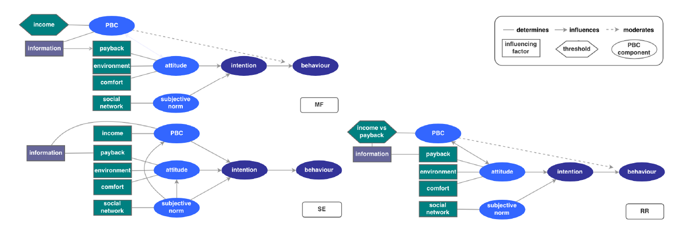
B: Sensitivity analysis
| Arch. | Variable | Value | Diffusion rate [0,1] | Energy production [106 GWh/yr] | CO\(_{2}\) savings [ktonne/yr] | Monetary savings [106 EUR] |
| MF | Income | \(r \in [0,1]\) | 0.910(0.004) | 316(1.1) | 3533.8(12.3) | 251(0.9) |
| Threshold | 0.00 | 0.956(0.002) | 325(0.9) | 3639.0(9.9) | 259(0.7) | |
| 0.05 | 0.923(0.003) | 320(0.9) | 3579.4(10.2) | 254(0.7) | ||
| 0.10 | 0.923(0.003) | 320(0.9) | 3579.4(10.2) | 254(0.7) | ||
| 0.20 | 0.782(0.003) | 286(1.1) | 3205.8(12.6) | 228(0.9) | ||
| SE | Importance | 0.00 | 0.564(0.004) | 253(1.6) | 2147.0(17.7) | 152(1.3) |
| Attitude | 0.20 | 0.748(0.004) | 253(1.6) | 2836.3(17.5) | 202(1.2) | |
| 0.40 | 0.835(0.004) | 283(1.4) | 3164.6(15.5) | 225(1.1) | ||
| 0.60 | 0.882(0.004) | 299(1.4) | 3351.5(15.3) | 238(1.1) | ||
| RR | PBS | 0.00 | 0.770(0.004) | 283(1.4) | 3172.2(15.5) | 226(1.1) |
| Barrier | 0.05 | 0.576(0.003) | 226(0.8) | 2534.5(9.4) | 180(0.7) | |
| 0.10 | 0.458(0.006) | 168(2.2) | 1876.2(24.9) | 133(1.8) | ||
| 0.20 | 0.020(0.002) | 4(0.5) | 51.6(5.8) | 4(3.7) | ||
| 50 random seed run per configuration | ||||||
| Importance PBC (Ipbc in Table 2 Equation (8)) | |||||
| 0 | 0.2 | 0.4 | 0.6 | ||
| Imp. Attitude | 0 | 0.564 | 0.564 | 0.564 | 0.564 |
| 0.2 | 0.748 | 0.748 | 0.748 | 0.748 | |
| 0.4 | 0.835 | 0.835 | 0.835 | 0.835 | |
| 0.6 | 0.882 | 0.882 | 0.882 | 0.882 | |
References
AJZEN, I. (1991). The theory of planned behaviour. Organizational Behaviour and Human Decision Processes, 50(2), 179–211. [doi:10.1016/0749-5978(91)90020-T]
ALEXANDER, P., Prestele, R., Verburg, P. H., Arneth, A., Baranzelli, C., Batista e Silva, F., Brown, C., Butler, A., Calvin, K., Dendoncker, N., Doelman, J. C., Dunford, R., EngstrÃűm, K., Eitelberg, D., Fujimori, S., Harrison, P. A., Hasegawa, T., Havlik, P., Holzhauer, S., HumpenÃűder, F., Jacobs-Crisioni, C., Jain, A. K., Krisztin, T., Kyle, P., Lavalle, C., Lenton, T., Liu, J., Meiyappan, P., Popp, A., Powell, T., Sands, R. D., Schaldach, R., Stehfest, E., Steinbuks, J., Tabeau, A., van Meijl, H., Wise, M. A. & Rounsevell, M. D. A. (2017). Assessing uncertainties in land cover projections. Global Change Biology, 23(2), 767–781.
AMELI, N. & Brandt, N. (2015). Determinants of households’ investment in energy efficiency and renewables: Evidence from the OECD survey on household environmental behaviour and attitudes. Environmental Research Letters, 10(4). [doi:10.1088/1748-9326/10/4/044015]
AN, L. (2012). Modelling human decisions in coupled human and natural systems: Review of agent-based models. Ecological Modelling, 229, 25 – 36. Modelling Human Decisions.
AXTELL, R. (2005). The complexity of exchange. The Economic Journal, 115(504), F193–F210. [doi:10.1111/j.1468-0297.2005.01001.x]
BALKE, T. & Gilbert, N. (2014). How do agents make decisions? A survey. Journal of Artificial Societies and Social Simulation, 17(4), 13: https://www.jasss.org/17/4/13.html. [doi:10.18564/jasss.2687]
BARRETEAU, O. (2003). The joint use of role-playing games and models regarding negotiation processes: characterization of associations. Journal of Artificial Societies and Social Simulation, 6 (2), 3: https://www.jasss.org/6/2/3.html.
BELL, A. R., Robinson, D. T., Malik, A. & Dewal, S. (2015). Modular abm development for improved dissemination and training. Environmental Modelling & Software, 73(Supplement C), 189–200.
BOER, C. (2015). Duurzaam dalfsen: the development of local initiatives and the path towards a carbon neutral municipality in 2025.
BOERO, R. & Squazzoni, F. (2005). Does empirical embeddedness matter? methodological issues on agent-based models for analytical social science. Journal of Artificial Societies and Social Simulation, 8(4), 6: https://www.jasss.org/8/4/6.html.
BOLDERDIJK, J. W., Steg, L., Geller, E. S., Lehman, P. & Postmes, T. (2013). Comparing the effectiveness of monetary versus moral motives in environmental campaigning. Nature Climate Change, 3(4), 413. [doi:10.1038/nclimate1767]
BRAVO, G., Vallino, E., Cerutti, A. K. & Pairotti, M. B. (2013). Alternative scenarios of green consumption in Italy: An empirically grounded model. Environmental Modelling & Software, 47, 225–234.
CBS (2009). Woononderzoek nederland 2009. Survey, Central Bureau voor de Statistiek, Rijksoverheid Nederland.
CESCHI, A., Dorofeeva, K., Sartori, R., Dickert, S. & Scalco, A. (2015). A simulation of households’ recycling attitudes based on the theory of planned behaviour. In Trends in Practical Applications of Agents, Multi-Agent Systems and Sustainability, (pp. 177–184). Springer
COLEMAN, J. (1990). Foundations of Social Theory. Belknap Press Series. Belknap Press of Harvard University Press.
DRESSLER, G. & Schulze, J. (2016). The challenges of implementing human decision making in agent-based models of natural resource use. In A.R. Sauvage S., J.-M. Sánchez-Pérez (Eds.), 8th International Environmental Modelling & Software Societ (iEMSs), Toulouse, France: http://www.iemss.org/sites/iemss2016/workshops.php
EDENHOFER, O., Pichs-Madruga, R., Sokona, Y., Seyboth, K., Kadner, S., Zwickel, T., Eickemeier, P., Hansen, G., Schlömer, S., von Stechow, C. et al. (2011). Renewable Energy Sources and Climate Change Mitigation: Special Report of the Intergovernmental Panel on Climate Change. Cambridge: Cambridge University Press. [doi:10.1017/CBO9781139151153]
EDMONDS, B. (2017). 'The Room Around the Elephant: Tackling Context-Dependency in the Social Sciences.' In Johnson, J., Nowak, A., Ormerod, P., Rosewell, B., Zhang, Y.-C. (Eds.), Non-Equilibrium Social Science and Policy: Introduction and Essays on New and Changing Paradigms in SocioEconomic Thinking, Berlin Heidelberg: Springer, pp. 195–208.
ELSAWAH, S., Guillaume, J. H., Filatova, T., Rook, J. & Jakeman, A. J. (2015). A methodology for eliciting, representing, and analysing stakeholder knowledge for decision making on complex socio-ecological systems: From cognitive maps to agent-based models. Journal of Environmental Management, 151(Supplement C), 500–516. [doi:10.1016/j.jenvman.2014.11.028]
FILATOVA, T., Polhill, J. G. & van Ewijk, S. (2016). Regime shifts in coupled socio-environmental systems: Review of modelling challenges and approaches. Environmental Modelling & Software, 75, 333–347.
FLACKE, J. & de Boer, C. (2016). An interactive GIS-tool for collaborative local renewable energy planning. In AGILE, Helsinki.
FORNI, M. & Lippi, M. (1997). Aggregation and the Microfoundations of Dynamic Macroeconomics. Oxford: Oxford University Press.
G., D. & Schulze, J. (2016). 'The challenges of implementing human decision making in agent-based models of natural resource use.' In A. R. Sauvage S., J.-M. Sánchez-Pérez (Ed.), 8th International Congress on Environmental Modelling and Software Society (iEMSs), Toulouse, France
GAMAL Aboelmaged, M. (2010). Predicting e-procurement adoption in a developing country: an empirical integration of technology acceptance model and theory of planned behaviour. Industrial Management & Data Systems, 110(3), 392–414.
GREENSTONE, M., Kopits, E. & Wolverton, A. (2013). Developing a social cost of carbon for us regulatory analysis: A methodology and interpretation. Review of Environmental Economics and Policy, 7(1), 23–46. [doi:10.1093/reep/res015]
GRIMM, V., Berger, U., DeAngelis, D. L., Polhill, J. G., Giske, J. & Railsback, S. F. (2010). The {ODD} protocol: A review and first update. Ecological Modelling, 221(23), 2760 – 2768.
HUDDART Kennedy, E., Krahn, H. & Krogman, N. (2015). Are we counting what counts? A closer look at environmental concern, pro-environmental behaviour, and carbon footprint. Local Environment, 20(2), 220–236. [doi:10.1080/13549839.2013.837039]
Intergovernmental Panel on Climate Change, I. (2015). Climate Change 2014: Mitigation of Climate Change, vol. 3. New York, NY: Cambridge University Press.
JAGER, W. (2000). Modelling Consumer Behaviour. Rijksuniversiteit Groningen.
JAGER, W., Janssen, M., De Vries, H., De Greef, J. & Vlek, C. (2000). Behaviour in commons dilemmas: Homo economicus and homo psychologicus in an ecological-economic model. Ecological Economics, 35(3), 357-379.
JANSSEN, M. A. (2017). The practice of archiving model code of agent-based models. Journal of Artificial Societies and Social Simulation, 20(1), 2: https://www.jasss.org/20/1/2.html [doi:10.18564/jasss.3317]
KASTNER, I. & Matthies, E. (2016). Investments in renewable energies by German households: A matter of economics, social influences and ecological concern? Energy Research and Social Science, 17, 1–9.
KAUFMANN, P., Stagl, S. & Franks, D. W. (2009). Simulating the diffusion of organic farming practices in two new EU member states. Ecological Economics, 68(10), 2580–2593. [doi:10.1016/j.ecolecon.2009.04.001]
KIRMAN, A. P. (1992). Whom or what does the representative individual represent? The Journal of Economic Perspectives, 6(2), 117–136.
KLABUNDE, A. & Willekens, F. (2016). Decision-making in agent-based models of migration: state of the art and challenges. European Journal of Population, 32(1), 73–97 [doi:10.1007/s10680-015-9362-0]
KNIVETON, D., Smith, C. & Wood, S. (2011). Agent-based model simulations of future changes in migration flows for Burkina Faso. Global Environmental Change, 21, S34–S40
Kniveton, D. R., Smith, C. D. & Black, R. (2012). Emerging migration flows in a changing climate in dryland Africa. Nature Climate Change, 2(6), 444–447. [doi:10.1038/nclimate1447]
KÖHLER, J., de Haan, F., Holtz, G., Kubeczko, K., Moallemi, E., Papachristos, G. & Chappin, E. (2018). Modelling sustainability transitions: An assessment of approaches and challenges. Journal of Artificial Societies and Social Simulation, 21(1), 8: https://www.jasss.org/21/1/8.html. [doi:10.18564/jasss.3629]
KOKS, E. E., Carrera, L., Jonkeren, O., Aerts, J. C. J. H., Husby, T. G., Thissen, M., Standardi, G. & Mysiak, J. (2016). Regional disaster impact analysis: comparing input–output and computable general equilibrium models. Natural Hazards and Earth System Sciences, 16(8), 1911–1924. [doi:10.5194/nhess-16-1911-2016]
MANSURY, Y. (2015). Bottom-up computational models of urban systems: In search of micro-foundations. Computers, Environment and Urban Systems, 54, 385 – 387.
MEYFROIDT, P. (2016). Approaches and terminology for causal analysis in land systems science. Journal of Land Use Science, 11(5), 501–522. [doi:10.1080/1747423X.2015.1117530]
MOGHAYER, S., Wissink, P., Arto, I., Filatova, T., Kovalevsky, D. V., Tol, R. & Niamir, L. (2016). Reporting on the development of the model database of complex climate-energy-economy system of models. EU FP7 COMPLEX Report D5.5: http://doc.utwente.nl/103382/
MOLLENHORST, G. (2015). Neighbour relations in the netherlands: new developments. Tijdschri voor economische en sociale geografie, 106(1), 110–119. [doi:10.1111/tesg.12138]
MOVE, D. (2014). Update of the handbook on external costs of transport. DG MOVE.
MUELDER, H. M. (2016). Household energy demand - behavioural changes and the role of information as an individual level barrier in transition to low carbon economy. Bachelor thesis, University of Twente, Enschede, Netherlands.
NAUCLÉR, T. & Enkvist, P.A. (2009). Pathways to a low-carbon economy: Version 2 of the global greenhouse gas abatement cost curve. McKinsey & Company, 192
PALMER, J., Sorda, G. & Madlener, R. (2015). Modelling the diffusion of residential photovoltaic systems in Italy: An agent-based simulation. Technological Forecasting and Social Change, 99, 106–131. [doi:10.1016/j.techfore.2015.06.011]
PARKER, D. (2018). Modelling complex urban environments. Specialist Conference Session.
PINDYCK, R. S. (2013). Climate change policy: What do the models tell us? Journal of Economic Literature, 51(3), 860–872. [doi:10.1257/jel.51.3.860]
POLHILL, G. & Gotts, N. (2017). How Precise Are the Specifications of a Psychological Theory? Comparing Implementations of Lindenberg and Steg’s Goal-Framing Theory of Everyday Pro-environmental Behaviour, (pp. 341–354). Cham: Springer International Publishing.
POLHILL, J. G., Parker, D., Brown, D. & Grimm, V. (2008). Using the ODD protocol for describing three agent-based social simulation models of land-use change. Journal of Artificial Societies and Social Simulation, 11(2), 3: https://www.jasss.org/11/2/3.html.
RAI, V. & McAndrews, K. (2012). Decision-making and behaviour change in residential adopters of solar pv. In Proc. of the World Renewable Energy Forum.
RAI, V., Reeves, D. C. & Margolis, R. (2016). Overcoming barriers and uncertainties in the adoption of residential solar PV. Renewable Energy, 89, 498–505. [doi:10.1016/j.renene.2015.11.080]
RAI, V. & Robinson, S. A. (2015). Agent-based modelling of energy technology adoption: Empirical integration of social, behavioural, economic, and environmental factors. Environmental Modelling & Software, 70, 163 – 177.
RAMOS, A., Labandeira, X. & Löschel, A. (2015). Pro-environmental Households and Energy Efficiency in Spain. Environmental and Resource Economics, 63(2), 367–393. [doi:10.1007/s10640-015-9899-8]
RICHETIN, J., Sengupta, A., Perugini, M., Adjali, I., Hurling, R., Greetham, D. & Spence, M. (2010). A micro-level simulation for the prediction of intention and behaviour. Cognitive Systems Research, 11(2), 181–193.
ROBBINS, R. W. & Wallace, W. A. (2007). Decision support for ethical problem solving: A multi-agent approach. Decision Support Systems, 43(4), 1571–1587. [doi:10.1016/j.dss.2006.03.003]
ROBERTS, S. C. & Lee, J. D. (2012). Using agent-based modelling to predict the diffusion of safe teenage driving behaviour through an online social network. In Proceedings of the Human Factors and Ergonomics Society Annual Meeting, vol. 56, (pp. 2271–2275). Sage Publications Sage CA: Los Angeles, CA
ROBINSON, D. T., Brown, D. G., Parker, D. C., Schreinemachers, P., Janssen, M. A., Huigen, M., Wittmer, H., Gotts, N., Promburom, P., Irwin, E. et al. (2007). Comparison of empirical methods for building agent-based models in land use science. Journal of Land Use Science, 2(1), 31–55. [doi:10.1080/17474230701201349]
ROBINSON, S. & Rai, V. (2015). Determinants of spatio-temporal patterns of energy technology adoption: An agent-based modelling approach. Applied Energy, 151, 273–284.
SCHLÜTER, M., Baeza, A., Dressler, G., Frank, K., Groeneveld, J., Jager, W., Janssen, M. A., McAllister, R. R., Müller, B., Orach, K. et al. (2017). A framework for mapping and comparing behavioural theories in models of social-ecological systems. Ecological Economics, 131, 21–35. [doi:10.1016/j.ecolecon.2016.08.008]
SCHWARZ, N. & Ernst, A. (2009). Agent-based modelling of the diffusion of environmental innovations — An empirical approach. Evolutionary Methodologies for Analysing Environmental Innovations and the Implications for Environmental Policy, 76(4), 497–511.
SCHWARZ, N., Kuhn, S., Seidl, R. & Ernst, A. (2016). Diffusion of water-saving technologies in private households: The innovation module of deephousehold. In Regional Assessment of Global Change Impacts, (pp. 339–346). Springer. [doi:10.1007/978-3-319-16751-0_43]
SILVA, E. A. & Wu, N. (2014). Dg-abc: An integrated multi-agent and cellular automata urban growth model. In Technologies for Urban and Spatial Planning: Virtual Cities and Territories, (pp. 57–92). IGI Global.
SMAJGL, A., Brown, D. G., Valbuena, D. & Huigen, M. G. (2011). Empirical characterisation of agent behaviours in socio-ecological systems. Environmental Modelling & Software, 26(7), 837–844. [doi:10.1016/j.envsoft.2011.02.011]
SOCIOVISION, S. (2004). Die sinus-milieus in Deutschland.
SOCIOVISION, S. (2007). Die sinus-milieus R in Deutschland 2007. See: http://www. sinussociovision. de
SOLOMON, S., Qin, D., Manning, M., Chen, Z., Marquis, M., Averyt, K., Tignor, M. & Miller, H. (2007). Contribution of working group I to the fourth assessment report of the intergovernmental panel on climate change, 2007.
STEG, L., Dreijerink, L. & Abrahamse, W. (2005). Factors influencing the acceptability of energy policies: A test of VBN theory. Journal of Environmental Psychology, 25(4), 415 – 425. [doi:10.1016/j.jenvp.2005.08.003]
STERMAN, J. D. (2000). Business dynamics: systems thinking and modelling for a complex world. McGraw-Hill Education.
STERN, N. (2016). Current climate models are grossly misleading: Nicholas stern calls on scientists, engineers and economists to help policymakers by better modelling the immense risks to future generations, and the potential for action. Nature, 530(7591), 407–410. [doi:10.1038/530407a]
STERN, P. C., Janda, K. B., Brown, M. A., Steg, L., Vine, E. L. & Lutzenhiser, L. (2016). Opportunities and insights for reducing fossil fuel consumption by households and organizations. Nature Energy, 1, 16043 EP –
TARIKU, M. B. (2014). Household energy demand in the Netherlands: Application of an agent-based model to assess the potential of carbon emission reduction. Master thesis, University of Twente, Enschede, Netherlands.
VAN Duinen, R., Filatova, T., Jager, W. & van der Veen, A. (2016). Going beyond perfect rationality: drought risk, economic choices and the influence of social networks. The Annals of Regional Science, 57(2), 335–369.
VERWAART, T. & Valeeva, N. I. (2011). An agent-based model of food safety practices adoption. In Emergent results of artificial economics, (pp. 103–114). Springer. [doi:10.1007/978-3-642-21108-9_9]
VOINOV, A. & Bousquet, F. (2010). Modelling with stakeholders. Environmental Modelling & Software, 25(11), 1268 – 1281. Thematic Issue - Modelling with Stakeholders.
VOINOV, A. & Shugart, H. H. (2013). ‘Integronsters’, integral and integrated modelling. Environmental Modelling & Software, 39(Supplement C), 149 – 158. Thematic Issue on the Future of Integrated Modelling Science and Technology [doi:10.1016/j.envsoft.2012.05.014]
WANG, M. & Hu, X. (2012). Agent-based modelling and simulation of community collective efficacy. Computational and Mathematical Organization Theory, 18(4), 463–487.
WEST, G. R. (1995). Comparison of input-output, input-output + econometric and computable general equilibrium impact models at the regional level. Economic Systems Research, 7(2), 209–227. [doi:10.1080/09535319500000021]
WILENSKY, U. & Evanston, I. (1999). Netlogo: Center for connected learning and computer-based modelling. North-Western University, Evanston, IL, (pp. 49–52).
WINDRUM, P., Fagiolo, G. & Moneta, A. (2007). Empirical validation of agent-based models: Alternatives and prospects. Journal of Artificial Societies and Social Simulation, 10(2), 8: https://www.jasss.org/10/2/8.html.
YU, L. & Gou, J. (2014). Multi-level agent model in the behaviour-intensive road intersection. In Intelligent Networking and Collaborative Systems (INCoS), 2014 International Conference on, (pp. 533–538). IEEE
YUN, S. & Lee, J. (2015). Advancing societal readiness toward renewable energy system adoption with a socio-technical perspective. Technological Forecasting and Social Change, 95, 170–181.