Loet Leydesdorff (2005)

Anticipatory Systems and the Processing of Meaning:
a Simulation Study Inspired by Luhmann's Theory of Social Systems

Journal of Artificial Societies and Social Simulation vol. 8, no. 2
<https://www.jasss.org/8/2/7.html>

To cite articles published in the Journal of Artificial Societies and Social Simulation, reference the above information and include paragraph numbers if necessary

Received: 29-Sep-2004    Accepted: 30-Jan-2005    Published: 31-Mar-2005

Abstract

Meaning can be communicated in addition to — and on top of — underlying processes of the information exchange. Meaning is provided to observations from the perspective of hindsight, while information processing follows the time axis. Simulations of anticipatory systems enable us to show how an observer can be generated within an information process, and how expectations can also be exchanged. Cellular automata will be used for the visualization. The exchange of observations among observers generates (a) uncertainty about the delineations in the observed system at each moment in time and (b) uncertainty about the dynamics of the interaction over time.

Keywords:

Anticipation, Autopoiesis, Social System, Incursion, Meaning

Introduction

1.1

In their foundational study of the simulation of social systems, Epstein and Axtell (1996) used the metaphor of 'growing artificial societies' on 'sugarscapes.' Human beings are then considered in terms of their observable behaviour. In general, multi-agent models begin with the specification of the activity at the nodes. The relations among the agents are modeled using a (potentially complex) function. The results of these simulations can be appreciated in terms of the quality of modeling the observable phenomena. The epistemological assumptions of this approach, however, have remained meta-biological: even if reflexivity is declared in the model, the exchange among agents is considered as a means to the ends of improving performance of agents in terms of 'survival' rates (e.g., Axelrod 1997; Dittrich et al. 2003).

1.2

Second-order social systems theory focuses on the dynamics of networks in terms of the links. What do the first-order exchanges of information mean for the evolving network system? The links represent interactions and can be considered as units of operation of the network. These operations stand analytically orthogonal to the agents operating at the nodes. The nodes and links remain structurally coupled in the co-variation (Maturana and Varela 1980). Given the perpendicularity of the reflexive angles, however, one can expect the perspectives of first-order and second-order systems theory to be very different (Simon 1969).

1.3

Interactions at the social level provide meaning to actions. According to Luhmann's (1984, 1997) theory of social systems, meaning processing can be considered as providing social and psychic systems with the ability to distinguish between actual and possible states of the system in terms of expectations. The communication of meaning is not a biological, but a cultural phenomenon (Luhmann 1986). Using Luhmann's definitions, however, there can be no meaningless information in meaning-processing systems. Information is defined by Luhmann (1984: 102f.) as a selection by the system, and not as uncertainty (Shannon 1948). The system, however, is defined as an operation at an interface with an environment. In this study, I show that simulation studies enable us to address this interface by considering expectations as a second-order landscape that can be distinguished from the first-order landscape of observable events. While the observable events develop by information processing along historical trajectories, the processing of anticipations by and among human beings can be considered as a selection mechanism that operates from the perspective of hindsight. The reflexive expectations import representations of future states into the present, that is, as a feedback mechanism against the arrow of time.

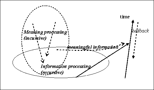
Figure 1. The incursive processing of meaning interacts with the recursive processing of information as a feedback mechanism. The result of the interaction can be considered as the production of meaningful information.

1.4

Systems which entertain models of their future states in the present, can be considered as anticipatory systems (Rosen 1985). I will first abstract the anticipatory model from its biological basis using Dubois's (1998) formalization. Second, a system which is both socially distributed and anticipatory will be decomposed into an observing system and a system under observation. In a third step, the quality of the observation is varied. The concept of anticipation is elaborated for a multi-agent system in terms of aggregation of and interaction among observations (Dubois and Sabatier 1998; Leydesdorff and Dubois 2004). The interaction among observers can then be distinguished from the interaction among observations. In a final section I provide a reflection about the relation between these simulations and Luhmann's social systems theory.

Derivation of the anticipatory model

2.1

The mathematical biologist Robert Rosen introduced the concept of anticipatory systems in 1985. Anticipatory systems were defined by this author as systems that contain a representation of the system itself (Rosen 1985; Dubois 2000). The internal representations can be used by the system for the anticipation because the system's parameters can be varied and recombined within the system. A biological system can use this degree of freedom for anticipatory adaptation, that is, by making a selection in the present among its possible representations in a next (phenotypical) exhibition. In electrical engineering, this model has been used to simulate the future behaviour of systems that contain delays in their operation (Dubois 2002).

2.2

In order to make these models relevant for social systems theory one has to specify how the communication among anticipatory agents can result in an anticipatory feed back at the systems level on the information processing among the (lower-level) agents. Let us perform this analysis step by step. I shall first specify the anticipatory model and then combine this mechanism with multi-agent modeling (that is, information processing) in a next step. Using a cellular automaton the generation of an observer will be made visible as a possible result of the interaction between the two mechanisms of anticipation and networking. After the specification of possible differences among observers in terms of their perspectives, I turn in the final parts of the study to the exchange of observations as a next-order level of the communication.

2.3

The study of anticipatory systems requires a model that is sufficiently complex to accommodate representations of the system within the system under study. These systems do no longer model an external world, but they entertain internal representations of their relevant environments in terms of the ranges of possible further developments. In other words, the possibility of anticipation in systems can be considered as an consequence of the complexity of the analytical model. This additional complexity is found by using the time dimension not as a (historical) given, but as another degree of freedom available to the system. This degree of freedom, that is, using different clocks, allows for active adaptation to changes in the environment through anticipation by inverting the arrow of time at some places more than (or differently from) others (Coveney and Highfield 1990).

2.4

When one simulates a process in discrete time steps, it is possible to evaluate the behaviour of a system over time using a forward or a backward appreciation of the differential equations. When these different formulations are provided with other appreciations, an anticipatory model can be generated. In general, the (continuous) differential equation dx/dt = f(x(t)) can be written as a difference equation (in discrete time) either as follows:

x(t + Δ t) = x(t) + Δ t f(x(t))

(1a)

or equivalently backward as:

x(t - Δ t) = x(t) - Δ t f(x(t))

(1b)

It follows that:

x(t) = x(t - Δ t) + Δ t f(x(t))

(1c)

The latter function allows for the following rewrite after one time-step Δ t:

x(t + Δ t) = x(t) + Δ t f(x(t + Δ t))

(1d)

Equation (1d) is different from Equation (1a) in terms of the time suffixes so that different classes of solutions can be expected. In Equation (1d) the state of a system at time (t + Δ t) depends on the state at the present time t, but also at the next moment in time (t + Δ t). The prediction 'includes' (or 'implies') its own next state. Dubois (1998) proposed that this evaluation be labeled incursion.

2.5

The behaviour of incursive models can be very different from recursive ones, even when the two models are based on the same differential equations. As will be demonstrated below, the incursive subroutine may balance the recursive one and thus counteract on instabilities (e.g., emerging bifurcations) in an evolving system. These effects of anticipations are highly relevant for understanding social systems because — as noted — social systems are driven both historically and by the expectations available and exchanged within them.

2.6

For example, the price of a commodity can be considered as its expected value on the market. The price is based both on an intrinsic value and on the feedback from the market system. The intrinsic value stems from the historical production given factor prices, while the feedback of the market originates in the present on the basis of the dynamics of current supply and demand. This economic system can be modeled using the anticipatory version of the well-known logistic or Pearl-Verhulst equation for the growth of biological systems (Pearl 1924; Verhulst 1847; Wolfram 2002: 198). However, the use of the traditional, that is, only forward, format of this model is ill-advised, since the two subdynamics of production and diffusion are then not sufficiently distinguished in terms of their dynamics over time. Production proceeds historically along the time axis, while diffusion takes place under competitive conditions in the present. The selection mechanism — in this case, the market — can be considered as an evolutionary feedback term on the historical development (Nelson and Winter 1982).

Historical developments and evolutionary feedback

3.1

The following model is known as the logistic map (Devaney 2003):

x(t) = a x(t-1) {1 - x(t-1)}

(2)

This equation can be used for modeling the growth of a population. The feedback term {1 - x(t)} inhibits further growth of the system represented by x(t) as the value of x(t) increases over time. This so-called 'saturation factor' generates the bending of the sigmoid growth curves of systems for relatively small values of the parameter (1 < a < 3). For larger values of a, the model bifurcates (at a ≥ 3.0) or increasingly generates chaos (3.57 < a < 4).

3.2

An anticipatory equivalent of the logistic equation can be formulated as follows:

x(t) = a x(t-1) {1 - x(t)}

(3)

In this model the selection pressure prevailing in the present is analytically independent of the previous state of the system that produced the variation. The recursion on x(t-1) can be considered as the historical subdynamic. As noted, technological systems which develop historically within an economy experience interaction with the market at each moment of time. In other words, the horizontal diffusion in the market stands in orthogonal relation to the historical development of the technology over time. The results of the interactions are continuously input to a next cycle that builds both recursively on the previous state and incursively experiences another feedback of the market at a next moment. However, the incursive subdynamics can be expected to have properties different from those of the recursive one (from which it was derived). For example, the anticipatory model based on the logistic equation does not exhibit bifurcation or chaos for larger values of the parameter a.

3.3

Let us first specify the model analytically and then — in a next section — demonstrate and discuss the behavioural differences by using cellular automata for the visualization of the effects in a social system which may contain both incursive (anticipatory) and recursive (historical) routines. The analytical reformulation of the Equation 3 proceeds as follows:

x(t) = a x(t-1) {1 - x(t)}	(3)
x(t) = a x(t-1) - a x(t-1). x(t)
x(t) + a x(t-1). x(t) = a x(t-1)
x(t){1 + a x(t-1)} = a x(t-1)
x(t) = a x(t-1) / {1 + a x(t-1)}	(4)

Equation 4 specifies x(t) as a function of x(t-1), but it remains equivalent to a model for incursion embedded in historical recursions as specified in Equation 3. In the case of pure incursion (that is, only environmental determination in the present as represented by the second term of Equation 3), one would no longer be able to produce a simulation because one would loose the historical axis of the system in the model. In other words, the anticipatory model containing both recursive and incursive factors imports the global or system's perspective into systems which are developing historically. The incursive term enriches the historically developing system with an orientation towards the future.

The simulations

4.1

Luhmann (1984: 240f.) defined social systems as consisting of communications and their attribution as action. The system of communication reproduces itself by linking communications to one another over time, while the attribution of these events as actions serves the observability of the system in historical time. The communications are operations which cannot directly be observed, but one can make inferences about them on the basis of the observable interactions among the agents (Luhmann 1984: 226). The communications and agents are structurally coupled and therefore the states of the agents can be used as indicators of the evolving communication processes among them.^[1] Let us begin the simulations at this observable end and consider social systems as based on exchange relations among actors.

4.2

Cellular automata enable us to display the dynamics of distributed (multi-agent) systems in terms of colours on the screen. Each point on the screen can be considered as an agent. Each agent is positioned by a horizontal and a vertical coordinate, that is, x and y. Different colours can be used to indicate the state of the various agents over time. However, the state of each agent and consequently the colour on the screen can be determined by the algorithms running at the level of the system and/or in local networks. In order to handle this mathematically, the value of each pixel (representing an agent) will be mapped in an array(x, y) with the size of the screen. In the simulations below, I use these two-dimensional array values and input them into the equations in a distributed mode, that is, at the randomly chosen place where change is generated.^[2] The screen colours are consequently updated.

4.3

For example, the logistic model reads in the two dimensions of the screen coordinates as follows:

(x, y)t = a (x, y)t-1 {1 - (x, y)t-1}

(2a)

This equation is used, for example, in line 130 of the computer program exhibited in Table 1.

4.4

An archive of executable program files, which will run under Microsoft Windows, may be downloaded from here. In order to enhance the transparency, I formulate the simulation models in standard BASIC.^[3] For example, the array from Equation 2a is defined in line 40 of Table 1 so that it can contain a representation of the screen in CGA-mode (200 x 320 pixels). The CGA-mode (line 10) was chosen in order to take full advantage of the visibility of the effects on the screen. A pixel — representing an agent — is selected randomly in lines 110 and 120. The results of the logistic evaluation of the corresponding array value (line 130) are brought to the screen in line 140: the pixel affected by the routine is thereafter repainted.

10 SCREEN 7: WINDOW (0, 0)-(320, 200): CLS 20 RANDOMIZE TIMER: a = 2.1 30 ' $DYNAMIC 40 DIM scrn(321, 201) AS SINGLE 50 FOR x = 0 TO 320 ' array and screen are filled in 60 FOR y = 0 TO 200 70 scrn(x, y) = .1: PSET (x, y), (10 * scrn(x, y)) 80 NEXT y 90 NEXT x 100 DO 110 x = INT(RND * 320) ' an array element is randomly 120 y = INT(RND * 200) ' selected 130 scrn(x, y) = a * scrn(x, y) * (1 - scrn(x, y)) 140 PSET (x, y), (10 * scrn(x, y)) 150 LOOP WHILE INKEY$ = '' 160 END

Table 1. Model for the logistic curve in BASIC (a = 2.1)

This code may be downloaded from here and run under Windows

Both the array and the screen are initially filled with a constant value in line 70; the screen is painted monochromatically. In the next loop (lines 100-150), a pixel is accessed randomly (lines 110-120), evaluated (line 130), and repainted accordingly (line 140). This transformation is performed continuously.

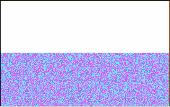
Figure 2. Resulting screen of Table 1 with bifurcation for a = 3.1

For the value of a = 2.1 (line 20), for example, the colour of the screen changes gradually because the distributed system exhibited on the screen goes through a transition.^[4] For a = 3.1, however, bifurcation is expected. This leads to a screen distributed randomly in two colours (Figure 2): when an agent is activated (lines 110-120), the colour on the screen changes into the alternative one at this place. Thus, the bifurcation leads to an oscillation between the two colours on the screen. For higher values of the parameter a, the system exhibits increasingly chaotic patterns of change.

4.5

Let us now turn to the anticipatory formulation of the logistic curve as specified in Equation 4 above. Table 2 provides the source code using a format similar to that of Table 1. However, following upon line 130 the screen is now split in two halves. The upper half of the screen (y > 100) is modeled using the incursive equation (Equation 4) in line 140, while the lower half remains recursive (Equation 2 in line 150 for y <= 100). The additional code in the first line enables the user to choose the parameter value interactively.^[5]

1 CLS : LOCATE 10, 10: INPUT 'Parameter value'; a 2 IF a > 4 THEN a = 4 ' prevention of overflow 10 SCREEN 7: WINDOW (0, 0)-(320, 200): CLS 20 RANDOMIZE TIMER 30 ' $DYNAMIC 40 DIM scrn(321, 201) AS SINGLE 50 FOR x = 0 TO 320 60 FOR y = 0 TO 200 70 scrn(x, y) = .1: PSET (x, y), (10 * scrn(x, y)) 80 NEXT y 90 NEXT x 100 DO 110 x = INT(RND * 320) 120 y = INT(RND * 200) 130 IF y > 100 GOTO 140 ELSE GOTO 150 ' split of screens 140 scrn(x, y) = a * scrn(x, y) / (1 + a * scrn(x, y)): GOTO 160 150 scrn(x, y) = a * scrn(x, y) * (1 - scrn(x, y)) 160 PSET (x, y), (10 * scrn(x, y)) 170 LOOP WHILE INKEY$ = '' 180 END

Table 2. Incursion and recursion in the case of the logistic curve

This code may be downloaded from here and run under Windows

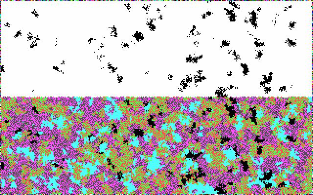
Figure 3. Upper half of the screen incursive, lower half recursive; a = 3.1

Figure 3 shows that the incursive simulation leads to a transition, while the representation of the recursive system in the lower half of the screen exhibits the same bifurcation as in Figure 2. The incursive model converges to a stable state (in this case, exhibited as white) because the incursive version of the logistic model {(ax / (1+ax)} grows towards unity with increasing values of x. In a mathematical formulation: Lim_x→∞ {ax/(1+ax)} = 1. A fixed point is reached independently of the starting value.

4.6

One can also combine the two subdynamics of incursion and recursion into a single screen by making the choice between the two models within the same system. The necessary changes in the codes are provided in Table 3. In this model the loops for the incursive or recursive routines are randomly assigned in line 130.

[...] 100 DO 110 x = INT(RND * 320) 120 y = INT(RND * 200) 130 IF RND > .5 GOTO 140 ELSE GOTO 150 140 scrn(x, y) = a * scrn(x, y) / (1 + a* scrn(x, y)) : GOTO 160 150 scrn(x, y) = a * scrn(x, y) * (1 - scrn(x, y)) 160 PSET (x, y), (10 * scrn(x, y)) 170 LOOP WHILE INKEY$ = '' 180 END

Table 3. Incursion and recursion alternating randomly, but using the same data set

This code may be downloaded from here and run under Windows

When the incursive model operates within a recursive system of which it is also a part, the incursive routine reduces the uncertainty produced by the recursive one. The recursive formulation can produce probabilistic entropy, but incursion drives steadily towards a transition in the long run.

4.7

The longer-term prevalence of incursion over recursion demonstrates the importance of accounting for expectations in models of cultural evolution since both subdynamics can be expected to occur in a social system. The emerging layers of social coordination can be expected to provide additional stabilities because of their selective capacity. Stabilization is a result of selections over time operating on (structural) selections at each moment of time. In other words, instantaneous selections on disturbances (which Luhmann sometimes calls 'irritations' or 'sensory sensations') can be selected recursively for stabilization over time and thereby structure (e.g., in the anticipations) can be retained. When a difference can recursively be processed, this may generate a reflexive stabilization.

4.8

By using incursion and therefore time as another degree of freedom, some stabilizations can further be selected for meta-stabilization or globalization (Mackenzie 2001). However, before moving to these next-order systems of communication, let us keep to the strategy of taking single steps and first simulate the emergence of an observer using an anticipatory model. Note that an observation can also be considered as the stabilization of a representation or, in other words, the specification of an expectation (Leydesdorff 2003).

The generation of an observer

5.1

Can the result of the interacting dynamics of a complex system that contains both incursive and recursive subroutines also be decomposed into an observing and an observed sub-system? In the model described in Table 4 and exhibited in Figure 4, the two routines of 'observed' and 'observing' are decomposed and thus an observer is generated.^[6] The upper half of the screen is reserved for the results of the incursive observations of the lower half of the screen, while the lower half exhibits the historical development of the observed system.

1 a = 3.3 10 SCREEN 7: WINDOW (0, 0)-(320, 200): CLS 11 LINE (1, 100)-(320, 100) 20 RANDOMIZE TIMER 30 ' $DYNAMIC 40 DIM scrn(321, 201) AS INTEGER 41 FOR x = 0 TO 320 42 FOR y = 0 TO 200 43 scrn(x, y) = INT(RND * 16) ' change to 16 colours 44 PSET (x, y), scrn(x, y) ' (see note 4) 45 NEXT y 46 NEXT x 50 DO 60 y = INT(RND * 200) 70 x = INT(RND * 320) 80 IF (x = 0 OR y = 0) GOTO 160 ' prevention of network errors 85 IF y > 100 GOTO 90 ELSE GOTO 100 90 scrn(x, y) = a * scrn(x, y-100) / (1 + a* (scrn(x, y-100) / 16)) 95 GOTO 140 ' paint upper screen 100 scrn(x, y) = a * (scrn(x, y) * (1 - (scrn(x, y)) / 16)) ' spread new value in the Von Neumann environment 110 scrn(x + 1, y) = scrn(x, y): scrn(x - 1, y) = scrn(x, y) 120 scrn(x, y + 1) = scrn(x, y): scrn(x, y - 1) = scrn(x, y) 140 PSET (x, y), ABS(scrn(x, y)) 160 LOOP WHILE INKEY$ = '' 170 END

Table 4. The generation of an observer by using incursion

This code may be downloaded from here and run under Windows

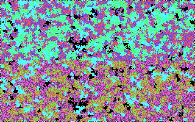
In order to generate an observable structure at each moment in time (because one cannot recognize patterns in the random observation of randomness), a small network effect was first added to the observed system (in lines 110-120 of Table 4). This network effect spreads the update in the lower-level screen in the local (Von Neumann) neighbourhood of the randomly affected cell. (The Von Neumann environment is defined as the cells above, below, to the right, and to the left of the effect.) Note that the network effect structures the system at each moment of time and locally, whereas incursion and recursion are defined over the time axis of the system.

5.2

The network effect enables us to appreciate on the screen the development of both the observed system and the relative quality of the observation depicted in the upper half of the screen. In order to exhibit more details on the screen, I will henceforth use the full range of 16 colours available in BASIC. This is achieved by changing the decimal base of the above simulations to the basis of 16 (line 43 of Table 4). Whenever necessary normalizations in the formulas for incursion and recursion are added (by dividing again by 16; for example, in lines 90 and 100).

5.3

A random attribution (line 60) is decisive (in line 85) for whether the recursive or the incursive routine is entered. The incursive routine (line 90) operates on the value of the corresponding array element in the lower half of the screen by evaluating scrn(x, y-100). The result of this evaluation is attributed to the upper half of the screen and to the corresponding array value of scrn(x, y). The effect is that an observer is generated as exhibited in Figure 4.

Figure 4. Incursion generates an observer in the top-level screen (a = 3.3)

5.4

In Figure 4, the parameter a is set at the value of a = 3.3 so that four colours are continuously produced by the logistic map operating in the lower half of the screen. The network effect in the Von Neumann neighbourhood (lines 110-120) adds observable structure to each bifurcation in two colours. The incursive top-half screen filters the black areas as an element of the observable structure. Under these conditions, however, the observer can distinguish only in black and white.

The generation of blind spots by different observers

6.1

The previous simulation has shown that an observer observes selectively, for example, only in black and white. By changing the parameter of the incursion, one can change the window of observation of an observer. Figure 5, for example, shows a similar simulation, but with the incursive parameter b set at half the value of the parameter for the recursion a (a = 3.2 and b = 1.6, respectively). The observer in this case observes detail in the structure in the lower half of the screen and different colours. However, the observer's reflections remain considerably less detailed than the representation of the observed system as exhibited on the lower half of the screen.^[7]

Figure 5. Incursion and recursion with different parameter values produce observers with potentially different positions and corresponding blind spots (a = 3.2 and b = 1.6).

1 CLS 2 LOCATE 10, 10: INPUT 'Parameter value for recursion (a) '; a 3 LOCATE 11, 10: INPUT 'Parameter value for incursion (b) '; b 4 IF a > 4 THEN a = 4 10 SCREEN 7: WINDOW (0, 0)-(320, 200): CLS 20 RANDOMIZE TIMER 30 ' $dynamic 40 DIM virtual scrn(321, 201) AS INTEGER 41 FOR x = 0 TO 320 FOR y = 0 TO 200 scrn(x, y) = INT(RND * 16) PSET (x, y), scrn(x, y) NEXT y NEXT x 50 DO 60 y = INT(RND * 201) 70 x = INT(RND * 321) 80 IF (x = 0 OR y = 0) GOTO 160 ' prevention of errors by 81 IF (x = 320 or y = 200) GOTO 160 ' effects at the margins 85 IF y > 100 GOTO 90 ELSE GOTO 100 90 scrn(x, y) = b*scrn(x,(y-100))/(1 + b*(scrn(x,(y-100))/16)) 95 GOTO 140 100 scrn(x, y) = a * scrn(x, y) * ((1 - (scrn(x, y)) / 16)) 110 scrn(x + 1, y) = scrn(x, y): scrn(x - 1, y) = scrn(x, y) 120 scrn(x, y + 1) = scrn(x, y): scrn(x, y - 1) = scrn(x, y) 140 PSET (x, y), ABS(scrn(x, y)) 160 LOOP WHILE INKEY$ = '' 170 END

Table 5. Incursion and recursion with different parameters

This code may be downloaded from here and run under Windows

By playing with the parameters, one can see that an observer perceives more detail when the parameter for the incursive routine is lower than for the recursive one. High values for the incursion parameter (b) drive the observing system into a more homogeneous state (because of the above noted limit transition in the formula), while higher values of the recursive parameter (a) drive the historically developing system towards more chaotic bifurcations.

Interactions among observers and interaction among observations

7.1

The possibility of generating observers with the different qualities of their respective observations raises the question of the possibility of interaction among the observers. What happens if the observers were able to observe also one another's observations? This would require that the observations are made available for communication in observational reports. In this study, I limit the interaction among observers to the simple interaction among and aggregation of observations. Human observers interact additionally by using more sophisticated mechanisms like human language or symbolically generalized media for the communication (Luhmann 1982 and 1997; Parsons 1963a and 1963b). This further extension is the subject of a next study (Leydesdorff 2005), but an expectation will be explicated in the final section of this study.

7.2

In the model of Table 6, two observers are differently defined in terms of the values of their respective parameters for the incursive routine. For the purpose of the presentation, the upper half of the screen is divided between them into a left and right half. Furthermore, one of the observers (the left hand one) is embedded in the recursive system under observation (as in the program of Table 3 above). The other observer remains external to the system under observation. Additionally, the two observers can differ in terms of the qualities of their observations by providing them with different parameters (b and c, respectively).

7.3

The observed system is represented in the lower left quadrant. The lower right quadrant is reserved for the averaged result of the observers observing each other's observations. The observers use their respective parameters for observing both the observed system and each other's observations.

1 a = 3.2: b = 1.6: c = 1.9 10 SCREEN 7: WINDOW (0, 0)-(320, 200): CLS 20 RANDOMIZE TIMER 30 ' $DYNAMIC 40 DIM scrn(321, 201) AS INTEGER 41 FOR x = 0 TO 320 FOR y = 0 TO 200 scrn(x, y) = INT(RND * 16) PSET (x, y), scrn(x, y) NEXT y NEXT x 50 DO 60 y = INT(RND * 201) 70 x = INT(RND * 321) 80 IF (x = 0 OR y = 0) GOTO 160 ' prevention of errors at the margins 81 IF (x = 320 OR y = 200) GOTO 160 IF x < 160 AND y >= 100 THEN N = 1 IF x >= 160 AND y >= 100 THEN N = 2 IF x < 160 AND y < 100 THEN N = 3 IF x >= 160 AND y < 100 THEN N = 4 SELECT CASE N CASE IS = 1 ' upper left screen scrn(x, y) = b * scrn(x, (y-100)) / (1 + b*(scrn(x, (y-100)) / 16)) PSET (x, y), ABS(scrn(x, y)) CASE IS = 2 ' upper right screen scrn(x, y) = c *scrn((x-160),(y-100))/(1 + c*(scrn((x-160),(y-100))/ 16)) PSET (x, y), ABS(scrn(x, y)) CASE IS = 3 ' lower left screen 100 IF RND > .5 GOTO 101 ELSE GOTO 110 101 scrn(x, y) = b * scrn(x, y) / (1 + b * (scrn(x, y)) / 16): GOTO 140 110 scrn(x, y) = a * scrn(x, y) * ((1 - (scrn(x, y)) / 16)) scrn(x + 1, y) = scrn(x, y): scrn(x - 1, y) = scrn(x, y) scrn(x, y + 1) = scrn(x, y): scrn(x, y - 1) = scrn(x, y) 140 PSET (x, y), ABS(scrn(x, y)) CASE IS = 4 ' lower right screen scrn(x, y) = c * scrn((x-160),(y+100))/(1 +c*(scrn((x-160),(y+100))/ 16)) 150 scrn(x,y) = (scrn(x,y)/2) + (b * scrn(x,(y+100)) / (1 + b*(scrn(x,(y+100))/16))) / 2 PSET (x, y), ABS(scrn(x, y)) END SELECT 160 LOOP WHILE INKEY$ = '' 170 END

Table 6. Two observers (incursion with b = 1.6 and c = 1.9) observe the same screen (recursion with a = 3.2) and each other. The left-side observer is additionally embedded (line 101).

This code may be downloaded from here and run under Windows

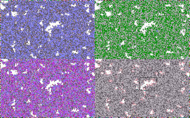
Figure 6. Two observers observing a single screen and each other (lower right screen). (Colours optimized in black and white by using the negative of the picture for the visualization.)

7.4

Figure 6 shows that the different values of the parameters for the observation lead to differently coloured perceptions of the system under observation. The embeddedness of the left-side observer makes no apparent difference from the representation in the upper-right quadrant upon visual inspection of these screens. The colour differences are generated only by the parameters of the observing systems. In this model, the observations of the observations are aggregated and the average of these two observations is exhibited in the lower right quadrant.

7.5

Both upper half screens provide less detail than the observed system (in the left bottom quadrant). The combination of the two observations is even poorer, but the boundaries of the (inverted) black spots exhibit an additional colour. In order to show this in black and white (printing), I added Figure 7 which amplifies the area indicated in Figure 6 by a factor of ten. The two observations differ somewhat and therefore the boundaries become uncertain when the observations of the observations are aggregated and averaged. (This is indicated with an additional shade of grey in Figure 7.)

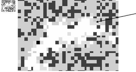
Figure 7. Part of Figure 6 ten times enlarged

7.6

In the next model (Figure 8), aggregation is replaced with interaction between the two observations. Whereas aggregation and the averaging of observations is based on interactions among observers, interaction among observations can be appreciated as meaning processing since this exchange is taking place in a next-order layer. However, the interaction and potentially meaningful coordination among observations remains structurally coupled to first-order observers (Luhmann 1999). Let us first study analytically the effects of introducing this interaction term.

[...] CASE IS = 4 ' lower right screen scrn(x, y) = c * scrn((x-160),(y+100))/(1 +c*(scrn((x-160),(y+100))/ 16)) 150 scrn(x, y) = (scrn(x, y)) * (b * scrn(x,(y+100)) / (1 + b*(scrn(x,(y+100))/16))) 151 scrn(x, y) = d * scrn(x, y) ' interaction parameter d PSET (x, y), ABS(scrn(x, y)) END SELECT 160 LOOP WHILE INKEY$ = '' 170 END

Table 7. The effect of interaction among the two observations

This code may be downloaded from here and run under Windows

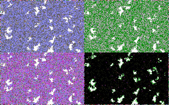
In order to see the pure effect of interaction — that is, without aggregation — I changed the plus sign in line 150 of Table 6 into a multiplication sign in Table 7. By adding a parameter d for the interaction (in line 151), one can then produce representations that are as rich in colours as the originally observed system (d = 0.2 exhibited in Figure 8) or as poor as an observer who only observes in black and white (d = 1.0).

7.7

My analytical point is that interaction is a non-linear operation which enables us to reconstruct the dynamics in and the various shades of the observed system by fine-tuning the interaction parameter. The two incursive observers first operate at random frequencies, but with different parameters. Consequently, an interaction among their observations contains a dynamic uncertainty that represents elements of the originally observed system that are lost in the individual reflections. The latter focus on the observable structure and thus reduce the complexity. The interaction of the reflections, however, opens a phase space of possible reconstructions of the observed system. This phase space can be appreciated at the social level if a cumulation of interactions would recursively be stabilized as another axis of the system.^[8]

Figure 8. Interaction effects among the two observations with interaction parameter d = 0.2

7.8

Given these parameters, all four (sub)screens visible in Figure 8 continue to reflect the network structure generated by the network effect in the observed system in the lower-left quadrant. The two observers, however, mainly observe structure. They tend to lose sight of the different colours of the arriving pixels generating the dynamics of change in the underlying screen (bottom left). The picture based on the interaction (in the lower-right quadrant) represents the ongoing dynamics of the system under observation by showing individual pixels that exist temporarily in colours other than the ones that reflect the network structure. These pixels are generated by dynamic frictions between the two observations which are out of phase because of (a) random differences in the update frequencies and (b) structural differences in the incursive parameters.

7.9

Figure 9 combines the two subdynamics of interaction and aggregation by assigning 40% of the visual effect to the interaction and 60% to the aggregation.

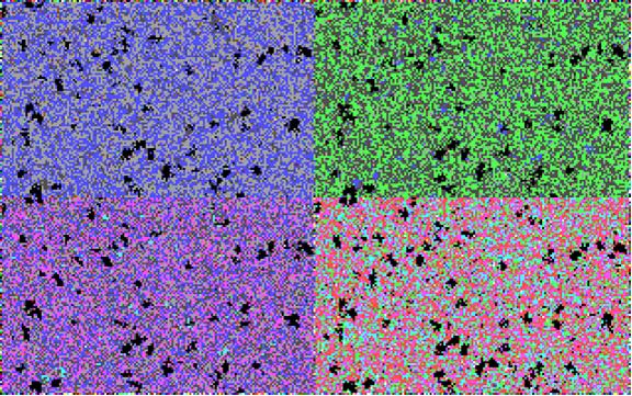
Figure 9. Interaction and aggregation of observations combined

The code may be downloaded from here and run under Windows

The resulting picture (in the lower right quadrant) shows the two effects described above: (a) the aggregation makes the observations uncertain in terms of the boundaries, and (b) the interaction shows the dynamics of the system under observation as pixels that temporarily light up on the screen. Because the two observers operate at random frequencies and with different parameters for the incursion, they are out of pace and entertain different representations. The latter effect provides a static uncertainty and the former a dynamic one.

7.10

In a next round of simulations the observers could be enabled to appreciate the effects of the aggregation and interaction of their observations. The next-order system of interacting observations can be further developed, for example, along emerging axes that stabilize new perspectives for the observation.^[9] In this study, however, I wished to show first that the simulation of social systems that exchange expectations is possible.

Discussion and further perspectives

8.1

Simulation models enable us to show visually what can be reasoned analytically, but the modeling requires the analyst to specify the assumptions with mathematical clarity. By taking the steps of anticipation, observation, aggregation, and interaction one by one, the construction of a social system of expectations could be made transparent. The dynamics of a social system, however, can be expected to remain complex and non-trivial because a social system contains a variety of different and interacting subdynamics.

8.2

The operation of second-order systems that process expectations cannot directly be observed. An observer is able to observe only the fingerprints that such operations leave behind. In a meaning-processing system the parameters of the observation are set by the system. An analyst first needs an interpretative frame for the observation of reflexive exchange processes (Luhmann 1984: 226; Leydesdorff 2003: 269). Yet, the exchange of meaning in relation to underlying information exchanges can be studied as a process of changing expectations by using simulation models. The simulations enable us to show the relevance of theoretical specifications about the dynamics of systems of expectations. For example, the differently expected effects of aggregation and interaction could be made visible.

8.3

One is able to distinguish analytically betewen anticipation by the system and information exchanges with its environments which provide the variation. The latent structure of social systems (Lazarsfeld and Henry 1968) can be expected to contain an internal subdynamic. Giddens (1979) used the word 'virtual' for this operation at the network level of what he called 'the duality of structure.' The operation over time can feedback on the structure at each moment of time. For example, the intellectual organization of a scientific specialty provides us with a system of expectations that does not coincide with the social organization of the field in terms of observable institutions like university departments and scientific journals (Whitley 1984). Another level of distributed control emerges within the social structure and its structure can be conjectured reflexively by the scholars trained in the specialty. But once in place, the intellectual organization may further develop, stagnate, or go into crisis without the departments being necessarily dissolved or the journals changing their publication patterns in the short term. The observable exchange relations process information historically, but the processing of meaning opens a global perspective on top of these 'instantiations' (Giddens 1984).

8.4

The instantiations of a social system indicate the existence of a system of expectations at a certain moment in time. For example, the institutions indicate continuation in history as a retention mechanism for the puzzles that the social systems have solved hitherto. When expectations can systematically operate upon one another, solutions at interfaces can be selected and sometimes stabilized. However, an analyst can only recognize the instantiations and institutions as sustaining a second-order dynamics of expectations if the anticipatory mechanisms of meaning exchange were first specified as relevant hypotheses. The observable variation can then be considered as provided with meaning by the agents and this process can also be reconstructed.

8.5

The historical observables themselves cannot provide sufficient control for the quality of the theorizing about meaning processing. The empirically observable phenomena inform us about cases that have occurred historically, but not about what could have occurred. In other words, one is not able to specify the uncertainty in the expectation on the basis of historical variations because the distribution of other possibilities is not 'given' in reality. However, some expectations about how the observable reality can be reconstructed by the reflexive observers may be more 'realistic' than others, that is, with reference to the reflected system. Simulations of social systems at the second-order level of expectations enable us to hypothesize selection mechanisms operating at the social level on theoretical grounds. Simulation studies can be considered as addressing a phase space of possible events which is different from the landscape of observable events. Thus, simulation studies of second-order exchange systems can contribute to sociological theorizing in a way very different from empirical observations.

8.6

Whereas empirical data enable the researcher to specify theoretical expectations, the simulations of incursive systems remain on the analytical side. The simulations enable us to improve the specificity of our analytical expectations. In this study, for example, relatively simple worlds containing both structural (network) elements and various subdynamics of change were generated. The system under observation could then be observed from different perspectives and implications for understanding the social character of observations could be specified.

8.7

The observers could first be distinguished in terms of the quality of their observations. One can focus on the communality in their observations. For example, the communality can be appreciated by comparing the observations. However, this comparison can also be made by the observers themselves using their incursive routines with the respective parameters for the observation. When these incursive routines were applied by the observers not only to the system under observation, but also recursively to each other's observations, two further perspectives could be made visible. First, an uncertainty in the delineations was induced at the margins of the structures visible on the screen. The two observers perceive somewhat differently, and therefore, the aggregate of their observations can be expected to contain an uncertainty. In other words, structures and delineations cannot be sharp in second-order exchanges. For example, this uncertainty among observations can reflexively lead to discussions about the quality of the observations (given that a code or language would be available for guiding the exchange).

8.8

Second, the dynamics of the observed system were brought back on stage by appreciating an interaction term among the observations. While the individual observers perceive the dynamics in the observed system, their focus remains on the structural network effects. However, the asynchronicity of the observations makes it possible to perceive dynamics in the interaction. In the lower right quadrant of Figure 9, this was visible as the single points that are generated with a different colour. In the two upper quadrants (representing first-order observers) these changes were perceived as ongoing changes within the range of the prevailing colours.

8.9

Among the two observers a fourth position is analytically possible (although beyond the scope of this study), notably one which inverts the time axis in the interaction among the observations by using another incursive loop. In the simulations of Figure 9, the lower right screen exhibited change and stability over time, but this process was followed along the historical axis of time. The reflection of this emerging order in relation to 'adjacent possibilities' (Kauffman 2000) assumes the exchange of meaning at the level of the social system. Such a system of meaning processing would need a symbolic layer like a code of the communication. A range of possible worlds might then be specifiable. This next-order loop can 'globalize' the historically stabilized systems of second-order expectations under specifiable conditions (Leydesdorff 1995). Luhmann (2002) in this context made reference to Husserl's (1929) phenomenology for indicating the notion of meaning occurring always within a horizon of possible meanings. In other words, the simulations studies of anticipatory systems provide us with a program for further research into the dynamics of second-order social systems.

Notes

¹Because Luhmann (e.g., 1986) defined agents in terms of 'consciousness,' the states of the agents should not be identified with behaviour.

²The extension to more than two dimensions is straightforward (Leydesdorff 2001).

³I used Microsoft's QBasic, but the programs can easily be adapted for higher or commercial versions of Basic, and for other languages. In Visual Basic the programs formulated in this paper can be imported as subroutines.

⁴In the compiled simulations, the values of the colours were augmented with five in order to use the brighter colours in the palette of QBasic.

⁵In order to prevent overflow while running this model, values of the parameter a larger than 4 are reset to a = 4 (in line 2).

⁶The subsystem entertaining the model of the system in the present state can be considered as an endogenous observer of the system's history. Endogenous means here that this observer remains a result of the network in which the observer effect is generated (Maturana 1978). One can consider this observer as an incursive subroutine of the complex system. Note that the metaphor is biological because this observer is not positioned refexively in a (next-order) communication among observers. The observer remains completely embedded and follows the development in the observed system reflexively.

⁷In the program in Table 5, the two parameters (a for the recursion and b for incursion, respectively) can be chosen by the user in the lines 2 and 3 of the routine. In Visual Basic the more sophisticated user interface would require the programming of an additional subroutine.

⁸The emergence of such a new dimension can, for example, be modeled as the effect of an unintended 'lock-in' (Arthur 1989 and 1994). I intend to elaborate on this further development of the social system in a next study.

⁹From a perspective along the time axis, these stabilizations can be considered as condensations of the expectations because of potential resonances among them (Smolensky 1986; Leydesdorff 1995).

References

ARTHUR W B (1989) Competing Technologies, Increasing Returns, and Lock-In by Historical Events. Economic Journal, 99. pp. 116-131.

ARTHUR W B (1994) Increasing Returns and Path Dependence in the Economy. Ann Arbor: University of Michigan Press.

AXELROD R (1997) The Complexity of Cooperation: agent-based models of competition and collaboration. Princeton: Princeton University Press.

COVENEY P and Highfield R (1990) The Arrow of Time. London: Allen.

DEVANEY R (2003) An Introduction to Chaotic Dynamical Systems, 2nd edition, Boulder, CO: Westview. pp. 33 ff.

DITTRICH P, Kron T and Banzhaf W (2003) On the Formation of Social Order: Modeling the Problem of Multi and Double Contingency following Luhmann. Journal of Artificial Societies and Social Simulation, 6 (1) https://www.jasss.org/6/1/3.html [21 September 2004].

DUBOIS D M (1998) "Computing Anticipatory Systems with Incursion and Hyperincursion." In Dubois D M (Ed.), Computing Anticipatory Systems: CASYS'97, AIP Proceedings 437. pp. 3-29.

DUBOIS D M (2000) "Review of Incursive, Hyperincursive and Anticipatory Systems — Foundation of Anticipation in Electromagnetism." In Dubois D M (Ed.), Computing Anticipatory Systems CASYS'99, AIP Proceedings 517. pp. 3-30.

DUBOIS D M (2002) "Theory of Incursive Synchronization of Delayed Systems and Anticipatory Computing of Chaos." In Trappl R (Ed.), Cybernetics and Systems, 1. Vienna: Austrian Society for Cybernetic Studies. pp. 17-22.

DUBOIS D M and Sabatier P (1998) "Morphogenesis by Diffuse Chaos in Epidemiological Systems." In Dubois D M (Ed.), Computing Anticipatory Systems: CASYS'97, AIP Proceedings 437. pp. 295-308.

EPSTEIN J M and Axtell R (1996) Growing Artificial Societies: Social Science from the Bottom Up. Cambridge, MA: MIT Press.

GIDDENS A (1979) Central Problems in Social Theory. London, etc.: Macmillan.

GIDDENS A (1984) The Constitution of Society. Cambridge: Polity Press.

HUSSERL E (1929) Cartesianische Meditationen und Pariser Vorträge. [Cartesian meditations and the Paris lectures.] Edited by S. Strasser. The Hague: Martinus Nijhoff, 1973.

KAUFFMAN S A (2000) Investigations. Oxford, etc.: Oxford University Press.

LAZARSFELD P F and Henry N W (1968) Latent structure analysis. New York: Houghton Mifflin.

LEYDESDORFF L (1995) The Operation of the Social System in a Model based on Cellular Automata. Social Science Information, 34(3). pp. 413-441.

LEYDESDORFF L (2001) Technology and Culture: The Dissemination and the Potential 'Lock-in' of New Technologies. Journal of Artificial Societies and Social Simulation, 4(3) https://www.jasss.org/4/3/5.html [Retrieved at 21 September 2004].

LEYDESDORFF L (2003) The Construction and Globalization of the Knowledge Base in Inter-Human Communication Systems. Canadian Journal of Communication, 28(3). pp. 267-289.

LEYDESDORFF L (2005) "Meaning, Anticipation, and Codification in Functionally Differentiated Social Systems." In Kron T, Schimank U, Winter L (Eds.), Luhmann simulated - Computer Simulations to the Theory of Social Systems, Münster, etc: Lit Verlag.

LEYDESDORFF L and Dubois D M (2004) Anticipation in Social Systems, Internation Journal of Computing Anticipatory Systems, 14. pp. 203-216.

LUHMANN N (1982) Liebe als Passion. Frankfurt a.M.: Suhrkamp.

LUHMANN N (1984) Soziale Systeme. Grundriß einer allgemeinen Theorie. Frankfurt a. M.: Suhrkamp.

LUHMANN N (1986) "The autopoiesis of social systems." In Geyer F, Van der Zouwen J (Eds.), Sociocybernetic Paradoxes, London: Sage. pp. 172-192.

LUHMANN N (1997) Die Gesellschaft der Gesellschaft. Frankfurt a.M.: Surhkamp.

LUHMANN N. (1999) "The Paradox of Form." In Baecker D (Ed.), Problems of Form, Stanford: Stanford University Press, pp. 15-26.

LUHMANN N (2002) "The Modern Sciences and Phenomenology." In Rasch W (Ed.), Theories of Distinction: Redescribing the descriptions of modernity. Stanford, CA: Stanford University Press. pp. 33-60.

MACKENZIE A (2001) The Technicity of Time. Time & Society, 10(2/3). pp. 235-257.

MATURANA H R (1978) "Biology of Language: the Epistemology of Reality." In Miller GA, Lenneberg E (Eds.), Psychology and Biology of Language and Thought. Essays in Honor of Eric Lenneberg. New York: Academic Press. pp. 27-63.

MATURANA H R and Varela, F (1980) Autopoiesis and Cognition: The Realization of the Living. Boston: Reidel.

NELSON R R and Winter S G (1982) An Evolutionary Theory of Economic Change. Cambridge, MA: Belknap Press of Harvard University Press.

PARSONS T (1963a) On the Concept of Political Power, Proceedings of the American Philosophical Society 107 (3). pp. 232-262.

PARSONS T (1963b) On the Concept of Influence. Public Opinion Quarterly 27 (1). pp. 37-62.

PEARL R (1924) Studies in Human Biology. Baltimore: William and Wilkins.

ROSEN R (1985) Anticipatory Systems. Oxford, etc.: Pergamon Press.

SHANNON C E (1948) A Mathematical Theory of Communication. Bell System Technical Journal, 27. pp. 379-423 and 623-356.

SIMON H A (1969) The Sciences of the Artificial. Cambridge, MA/London: MIT Press.

SMOLENSKY P (1986) "Information Processing in Dynamical Systems: Foundation of Harmony Theory." In Rumelhart D E, McClelland J L, and the PDP Research Group (Eds). Parallel Distributed Processing. Cambridge, MA/ London: MIT Press, Vol. I. pp. 194-281.

VERHULST P-F (1847) Deuxième mémoire sur la loi d'accroissement de la population, Mém. de l'Academie Royale des Sci., des Lettres et des Beaux-Arts de Belgique, 20. pp. 1-32.

WHITLEY R D (1984) The Intellectual and Social Organization of the Sciences. Oxford: Oxford University Press.

WOLFRAM S (2002) A New Kind of Science. Champaign, IL: Wolfram Media.

Return to Contents of this issue

© Copyright Journal of Artificial Societies and Social Simulation, [2005]