
Alan G. Isaac (2008)
Simulating Evolutionary Games: A Python-Based Introduction
Journal of Artificial Societies and Social Simulation
vol. 11, no. 3 8
<https://www.jasss.org/11/3/8.html>
For information about citing this article, click here
Received: 12-Feb-2008 Accepted: 01-Apr-2008 Published: 30-Jun-2008

 Abstract
1.1
Computer simulation of social and economic interactions has been gaining adherents for more than two decades.
Contemporary researchers often promote simulation methods as a “third way” of doing social science,
distinct from both pure theory and from statistical exploration (Axelrod 1997).
While many methodological questions remain areas of active inquiry,
especially in the realms of model robustness and model/data confrontations,
researchers have been attracted by the ease with which computational methods can shed light on intractable theoretical puzzles.
Some researchers have gone so far as to argue that pure theory has little left to offer—that for social science to progress, we need simulations rather than theorems (Hahn 1991).
1.2
One specific hope is that simulations will advance social science by enabling the creation of more realistic models.
For example, economists can build models that incorporate important historical, institutional, and psychological properties that “pure theory” often has trouble accommodating,
including learning, adaptation, and other interesting limits on the computational resources of real-world actors.
Another specific hope is that unexpected but useful (for prediction or understanding) aggregate outcomes will emerge from the interactions of autonomous actors in agent-based simulations.
These hopes are already being met in many surprising and useful ways (Bonabeau 2002).
1.3
Simulations are considered to be agent-based when the outcomes of interest result from the repeated interaction of autonomous actors, called ‘agents’.
These agents are autonomous in the sense that each agent selects actions from its own feasible set based on its own state.
An agent is often a stylized representation of a real-world actor:
either an individual, such as a consumer or entrepreneur,
or an aggregate of individuals,
such as a corporation or a monetary authority (which may in turn be explicitly constituted of agents).
1.4
Substantial research in agent-based simulation (ABS) has been conducted in a variety of general purpose programming languages,
including procedural languages such as Fortran, C, or Pascal;
object oriented languages such as Objective-C, Smalltalk, C++, or Java;
very-high level matrix languages such as MATLAB or GAUSS;
and even symbolic algebra languages such as Maple or Mathematica.
There are also a variety of special purpose toolkits for ABS,
including SWARM and MAML (built in Objective-C);
Ascape, NetLogo, and Repast (built in Java);
and many others (Gilbert and Bankes 2002).1
In addition,
there are a few efforts at general environments in which a variety of ABS experiments can be run.
(Bremer's GLOBUS model, Hughes's IFs model, and Tesfatsion's Trade Network Game model are salient examples.)
Researchers occasionally express the hope that one of these might emerge as a lingua franca for ABS research (Luna and Stefansson 2000).
Working against this,
as others note,
are the interfaces of capable toolkits and environments,
which are often as difficult to master as a full-blown programming language (Gilbert and Bankes 2002).
A variety of languages and toolkits remain in use,
and this seems likely to persist,
along with efforts to assess their relative utility (Railsback et al. 2006).
1.5
This paper explores the use of Python as a language for ABS experiments.
Python is a very-high-level general-purpose programming language
that is suitable for a range of simulation projects,
from class projects by students to substantial research projects.
In the face of the plethora of alternatives,
an additional ABS research language may seem otiose.
However this paper shows that the Python programming language offers a natural environment for agent-based simulation
that is appropriate for both research and teaching.
1.6
This paper illustrates that suitability by quickly and simply developing a toolkit
that can be applied to a classic ABS model:
the evolutionary iterated prisoner's dilemma.
This application,
which is familiar to social scientists and illustrative of key needs in ABS research,
serves to illustrate some virtues of Python for such simulation projects.2
The core goals of the paper naturally imply a substantial tutorial component:
an introduction to agent-based simulation for those new to the area,
an introduction to simulation of the evolutionary iterated prisoner's dilemma,
and a very narrowly focused introduction to the Python programming language.
Since code reuse and extensibility are crucial components of simulation projects,
we also show how to extend a basic simulation toolkit
to explore the importance of topology, payoff cardinality, and strategy evaluation for evolutionary outcomes.
1.7
The iterated prisoner's dilemma (IPD) is familiar to many social scientists,
and many ABS researchers have implemented some version of the IPD as an exercise or illustration.
Readers with ABS backgrounds will be able to appreciate how
simple, readable, and intuitive our Python implementation proves
when compared to similar projects implemented in other languages.3
This is a key reason to use Python for ABS research and teaching:
with a little care from the programmer and an extremely modest understanding of Python by the reader,
Python code can often be as readable as pseudocode.
This is no accident:
readability is an explicit design goal of the Python language.
1.8
The core objective of the paper is to enable students, teachers, and researchers
immediately to begin social-science simulation projects in a general purpose programming language.
We achieve this by pursuing three related goals.
First, we offer an introduction to the object-oriented modeling of agents,
which is a crucial component of agent-based simulation.
Second, we elaborate a simple yet usable toolkit that we apply to a classic ABS model:
an evolutionary iterated prisoner's dilemma.
The speed and ease with which this prototype is developed
supports our claim that ABS research and teaching find a natural ally in the Python programming language.
Finally, we illustrate code reuse and extensibility
by extending our basic toolkit in two directions,
exploring the importance of topology and of payoff cardinality for evolutionary outcomes.
2.1
This section provides a very brief introduction to object-oriented programming and
its relationship to agent-based simulation.
It also provides a similarly brief introduction to aspects of the Python programming language
that facilitate ABS research.
2.2
Agent-based simulation is most naturally approached with object-oriented programming languages.
In order to illustrate this natural relationship, we need a little vocabulary.
An object is a collection of characteristics (data) and behavior (methods).
In a game simulation, for example,
a player object may have a move history as data and a method for producing new moves.
We will call a computer program ‘object-based’
to the extent that data and methods tend to be bundled together into useful objects.
2.3
Many researchers consider models of interacting agents to be naturally object-based.
For example,
a player in a game is naturally conceived in terms of that individual player's characteristics and behavior.
We may therefore bundle these together as the data and methods of a player object.
(The next section presents an example.)
2.4
In the present paper,
we will consider object-based code to be “object-oriented” when it relies on encapsulation.4
Code relies on encapsulation when objects interact via interfaces that conceal implementation details:
users of an object rely on its interface,
without detailed knowledge of how the object produces its behavior.
For example, we will design a player object
such that we can ask for its next move simply by communicating with its move method,
without worrying about how that method is implemented.
Specifically,
we need not worry about whether the player owns the data used to produce the move,
or even whether the player delegates the selection of the move to some other agent.
2.5
Given this highly simplified taxonomy,
we can say object-oriented programming (OOP) is possible in most computer languages.
It is a matter of approach and practices:
OOP focuses on defining encapsulating objects and determining how such objects will interact.
Yet it is also the case that some languages facilitate OOP.
We say a programming language is object-oriented to the extent that it facilitates object-oriented programming.
2.6
Key facilities of any OOP language are inheritance and polymorphism.
Inheritance is essentially a useful way to implement the old practice of code reuse:
one class of objects can inherit characteristics (data) and behavior (methods) from another class.
This allows common data and methods to be coded at a single location,
reducing coding errors and facilitating program maintenance and debugging.
In practice,
we often create specialized classes that inherit from more general classes,
making it easy to compare the implications of various behavioral specializations.
Inheritance proves to be an extremely powerful way to reuse existing code,
and it often facilitates writing simpler, more robust, and easier to understand code.
Part of the resulting simplicity arises through ‘polymorphism',
as when a common method call is made to distinct classes that provide divergent responses.5
For example,
all player classes implement a move method,
but some players base their move selection on their past playing experience and others do not.
For an object to participate as a player in a particular game,
it must respond appropriately to certain messages.
For example, it must have a move method that accepts certain arguments and returns appropriate values.
However,
we need not know anything about the inner workings of the player's move method;
how a player moves can vary by player type.
(Subsequent sections provide examples.)
2.7
The phenomenologically salient actors of social science will often be natural objects in our simulation models.
This adds intuitive appeal to our simulation models:
the actors in our artificial world are these objects.
The interactions of these autonomous units produce the model outcomes,
suggesting analogies to the ways in which real-world actors produce real-world outcomes.
This aspect of OOP can facilitate production of sensible models
and almost certainly helps with communication—two big advantages in a relatively new area of research.6
2.8
Researchers naturally attend to productivity when choosing a programming environment.
Students and teachers are particularly interested in ease of use,
cost, and the availability of good documentation and support groups.
The choice of programming language will therefore be very personal,
responding to cost, to individual modes of thinking, and to existing human capital.
That said, Python's combination of ease of use, power, and readability
constitute an attractive environment.
This section provides an overview of some of these features.
(Appendix B includes guidance for installing and running Python.)
2.9
Python is a young language:
version 1 was released in 1994,
and the very popular version 2.2 had its final release in 2003.
Despite its youth,
Python is considered stable and robust,
with around a million users (Lutz 2007).
Python is open-sourced under the liberal Python License,
which ensures that it can be freely used (even in commercial projects).
The Python Software Foundation protects the Python trademark,
funds Python related development,
and provide extensive documentation for both beginners and advanced users.
Python's unusally clear syntax and ease of use has made it
increasingly popular in introductory computer science classes.
At the same time, Python's power, flexibility, true object orientation, and ready integration
with other languages have given Python a growing presence in business and scientific computing.
These are the same features that will underpin the simplicity and readability of the
game simulations presented below.
2.10
Many researchers claim that OOP languages facilitate ABS modeling.
Among the OOP languages,
Python is notable for its readability,
ease of use,
and natural syntax—all of which facilitate rapid learning and easy prototyping.
This does not constitute an argument that Python is the “best” language for agent-based simulation,
whatever that might mean;
it simply highlights a few features that make Python an attractive language for students,
teachers,
and researchers who have not already made a language commitment.
No single feature makes Python unique,
but together they add up to an attractive combination of power and ease of use.
Here are a few salient considerations.
A few powerful, flexible, and extremely easy to use data structures are built-in, in the sense that Python always makes them available. Here we mention the two sequence data types (list and tuple) and one mapping type (dict).9
Sequence data types are indexed collections of items, which may be heterogeneous. Lists and tuples are sequence types that are ubiquitous in Python programming. An empty list can be created as [] or as list(); an empty tuple can be created as () or as tuple(). A populated list or tuple can be created with a comma separated listing of its elements: [1,'a'] is a two element list (with heterogeneous elements); (1,'a') is a two element tuple (with the same elements); and [(3,3), (0,5)] is a list containing two tuples, which each contain two elements.
Tuples are immutable: they cannot be changed after they are created. Lists are mutable: they can grow as needed, and elements can be replaced or deleted. (See Appendix B for more details.)
Sequences can be used for very convenient loop control: Python's for statement iterates over the items of a sequence. For example, if seq is a list or tuple, the following code snippet prints a representation of each item in seq:
for item in seq:
    print item
The dictionary is the basic Python mapping data type (resembling hash tables or associative arrays in other languages). A dictionary is a collection of key-value pairs, where the value can be retrieved by using the key as an index. If x=dict(a=0,b=1) then x['a'] returns the value 0 and x['b'] returns the value 1. The same dictionary can be created from a sequence of 2-tuples: x=dict( [('a',0), ('b',1)] ).
A few dozen very useful functions are built-in, in the sense that Python always makes them available. Examples include list, tuple, and dict, which are discussed above. The user does not need to import any standard library modules to access built-in functions. We will mention one more at this point: range.
If i is a nonnegative integer, then range(i) creates a list of the first i nonnegative integers. It is idiomatic in Python to use range for loop control. For example,
for i in range(10):
    print i
Python uses very powerful and easy to read syntax for the creation of data structures. Rather than traditional looping constructs, “generator expressions” are often preferred for producing lists and tuples. Generator expressions are perhaps best introduced by contrast with traditional practices.
Let players be a collection of players, each of whom has a playertype attribute, and suppose we want to produce a corresponding tuple of playertypes. Here is a (fairly) traditional approach to this problem:
ptypes = list()
for player in players:
    ptypes.append(player.playertype)
ptypes = tuple(ptypes)
In this traditional approach, we create an empty list, to which we sequentially append the playertype type of each player, and we finally create a tuple corresponding to the list of playertypes.11 As an alternative approach, we can accomplish the same thing more elegantly and efficiently with a generator expression:
ptypes = tuple( player.playertype for player in players )
This iterates through the generator (player.playertype for player in playerlist) to populate a tuple of player types, one playertype for each player.12 (In contrast with the first approach, we side-step the creation of a temporary list.) The expression on the right reads very naturally: create a tuple that contains the player's playertype for each player in players. This is a remarkably readable and compact way to generate this new tuple's elements.
2.11
The following more technical considerations may interest an instructor or a new researcher
who is considering the use of Python for agent-based modeling.
Other readers can skip this section.
2.12
Other important features of Python—exception handling, support for unit testing, support for multiple inheritance, support for metaclasses, support for metaprogramming (via descriptors such as decorators and properties), support for simple but sophisticated operator overloading, and memory conserving features such as slots—prove useful in advanced applications.
These issues are beyond the scope of the current paper.
3.1
When discussing agent-based simulations,
nothing substitutes for actual code,
so we will now implement a very simple game.
We initially eschew game theoretic considerations:
our two players will randomly chose their moves and ultimately receive the payoffs determined by the game.
(See Appendix B for suggestions on how to run the following code.)
3.2
This section provides an introduction to Python classes.
We therefore begin by defining a fairly trivial class.
A class definition provides a general description of the data and methods of a new type of object,
and accordingly our definition of the RandomMover class provides a general description of our first game players.
A RandomMover has no data and a single method, named move.
We will soon create our first game players as “instances” of this RandomMover class,
but first we will examine the class definition.
(Readers familiar with class and function definitions can skim the next few paragraphs.)
class RandomMover:
    def move(self):
        return random.uniform(0,1) < 0.5
3.3
Note that a class definition starts with the keyword class,
followed by the name (RandomMover) that we are giving the class,
followed by a colon.16
So the line class RandomMover: is our class-definition header:
it begins our definition of the RandomMover class,
which is completed by the indented statements that follow.
(Blocks are always defined in Python by level of indentation
and never by the use of braces.)
3.4
The body of this class definition is a function definition,
which defines the only behavior of a RandomMover instance.
When asked to move,
a RandomMover instance will return a random move,
based on a draw from a standard uniform distribution.
3.5
A function definition starts with the keyword def,
followed by the name (move) that we are giving the function,
followed by parentheses that enclose any function parameters,
followed by a colon.
So the line def move(self): is our function definition header;
it begins our definition of the move function,
which is completed by the indented statement that follows.
This function has one argument,
which is called self for reasons that we now discuss.
3.6
Functions defined in the body of a class definition are called ‘methods’.
Methods define the behavior of instances of that class.
When an instance receives a method call,
Python always provides as an implicit first argument the instance itself.
(This is likely to sound obscure to a reader with no OOP background,
but it should be clear by the end of this section.)
Therefore it is conventional to name this first argument self.
Note that even when the body of a method does not make use of the self argument,
as illustrated by this introductory example,
we still must include the self argument in the method definition.17
3.7
Since Python uses indentation to delimit code blocks,
we must indent our function-definition header to make it part of the class definition.
Similarly, the body of the function definition is given an additional level of indentation.
In this case, the body of the function is a single statement: return random.uniform(0,1) < 0.5.
When this return-statement is executed,
the expression random.uniform(0,1) < 0.5 is evaluated,
and the resulting value is returned by our move method.
This value is computed as follows.
The expression random.uniform(0,1) evaluates to a draw from a standard uniform distribution,
so it is a “random” number between zero and one.18
It is compared to the number 0.5.
The inequality comparison value is either True or False.
In what follows,
a player must choose between two behaviors,
which we call “defection” (represented by True or 1) or “cooperation” (represented by False or 0).
These behaviors are discussed in more detail in the Prisoner's Dilemma section.
3.8
We will now play a simple game.
We begin by creating a payoff matrix for the game.
(Note that we include in the code a comment to that effect:
the hash mark (#) is a comment marker, signalling that the rest of the line is commentary rather than code.)
We will use the payoff matrix used in Scodel et al. (1959) and in many subsequent studies.
(In subsequent sections, we will consider the role of the payoff matrix in much more detail.)
The payoff matrix is constructed from lists and tuples (as discussed above).
The assignment PAYOFFMAT = [ [(3,3),(0,5)] , [(5,0),(1,1)] ] creates a list containing two lists,
each of which contains two tuples.
These tuples hold the move-based payoffs for two players.
For example, the tuple (3,3) gives the payoffs to the players if both cooperate:
each player gets a payoff of 3.
    ## GAME: RandomMover
    # create a payoff matrix and two players
    PAYOFFMAT = [ [(3,3),(0,5)] , [(5,0),(1,1)] ]
    player1 = RandomMover()
    player2 = RandomMover()
    # get a move from each player
    move1 = player1.move()
    move2 = player2.move()
    # retrieve and print the payoffs
    pay1, pay2 = PAYOFFMAT[move1][move2]
    print "Player1 payoff: ", pay1
    print "Player2 payoff: ", pay2
3.9
We next create two RandomMover instances,
which we name player1 and player2.19
Recall that a class definition provides a general description of a new kind of object,
and we use this definition to create instances of this new kind of object.
We can assign a RandomMover instance to the name player1 like this: player1 = RandomMover().
We say that each player “instantiates” the RandomMover class.
3.10
Next we get moves from player1 and player2
by calling the move method of each player.20
Using these moves and the payoff matrix,
we calculate the payoff for each player.
(True is equivalent to the integer 1,
and False is equivalent to the integer 0.)
Finally we print the results of playing this game.
(A comma separates items to be printed,
so the first print statement prints two items:
the descriptive string delimited by quotes,
and the value of the player1 payoff.)
3.11
In the previous section,
we defined the RandomMover class to have a built in probability of defection of 0.5.
If we repeatedly play the game of that section,
we will discover the average payoff implied by this strategy.
Much more informative would be the average payoff for each of a variety of strategies.
It would be senseless to create a new class for each strategy.
Instead, we will create a class that can produce instances that have different strategies.
We will call this class RandomPlayer.
This section illustrates what happens when RandomPlayer instances
with various defection probabilities play against each other.
3.12
In the previous section we coded a simple two-player game:
we ran the game and computed player payoffs based on a payoff matrix.
Our desire to run such games repeatedly for a variety of player strategies
suggests that a game is a natural object in our project.
In this section,
the games played will be instances of a SimpleGame class.
3.13
Consider the following initial design,
which allows for a game object and player objects to interact.
A SimpleGame instance will have as data a list of players and a payoff matrix,
and it will also have a history attribute to hold the game history.
A game will have a run method (to run the game)
and a payoff method (to compute player payoffs based on player moves and the payoff matrix).
3.14
The design stage is the time to plan for interactions between a game and its players.
We must decide on our interfaces,
which are set the basic rules for how games and players can interact.
To make the SimpleGame class useful for later simulations,
it will not only ask each player for a move
but it will offer each player a chance to record the game (itself).
Although we do not plan on doing any recording in our initial games,
we will define our RandomPlayer class to match this behavior:
it not only must have a move method but also must have a record method.
(In addition, a SimpleGame will always pass itself when calling a player method,
so each of these methods must accept a game as an argument.)
A summary of the proposed data and methods for these two classes follows.
3.15
Each RandomPlayer has a single data attribute:
its probability of defection, p_defect, which can differ by player.
We will now use RandomPlayer instances to play our SimpleGame.
Players of a SimpleGame must respond to certain messages (i.e., method calls).
This implies a general interface requirement for any player of a SimpleGame:
the player must respond to move and record method calls.21
The RandomPlayer class therefore includes move and record methods.
3.16
The RandomPlayer class has much in common with the RandomMover class:
by default it moves just like a RandomMover,
and its record method does nothing.
Let us focus on the changes.
First the big change:
notice that the RandomPlayer class defines a method named __init__.
This is a special name,
reserved for the method that does the ‘initialization’ of a new instance.22
Typically, initial values of instance attributes are set during initialization.
The __init__ method of a RandomPlayer has a single responsibility:
to set the initial value of the player's p_defect attribute.
Since each RandomPlayer instance will have its own probability of defection,
we say that p_defect is an “instance attribute”.
We provide a default value of 0.5,
but an instance can always be created with a different value.23
class RandomPlayer:
    def __init__(self, p=0.5):
        self.p_defect = p
    def move(self, game):
        return random.uniform(0,1) < self.p_defect
    def record(self, game):
        pass
3.17
The function-definition headers for the move and record methods reflect
our design decisions, discussed above.
Whenever a SimpleGame calls the move or record method of a player,
it will pass itself.
In later sections,
this will prove a useful feature of the SimpleGame class.
This later utility determines the signature of these methods in our RandomPlayer class.
That is,
we design this illustrative RandomPlayer class for interactions with a more generally useful game class.
3.18
The move method of a RandomPlayer is largely unchanged.
However since we want our RandomPlayer instances to play a SimpleGame,
we must add a new argument, which we name game.
The new argument simply provides a consistent interface,
anticipating that a game will always pass itself when it calls a player's method.
The record method also reflects this interface decision,
although the record method literally does nothing.
(Python uses the keyword pass to indicate “do nothing”.)
This method exists solely to accommodate our interface design—that is,
to allow a RandomPlayer to play a SimpleGame.
3.19
It is time for some slightly heavier lifting.
SimpleGame is the most complex class we introduce in this paper,
but it includes many now familiar components.
Specifically, the design of its methods
parallels the code we used to run our previous game simulation.
One benefit of the care with which we will approach the design
of our SimpleGame class
is that we can continue to use it throughout this paper.
3.20
The class definition begins in a familiar way.
After the class-definition header (class SimpleGame:),
we define an __init__ method to initialize newly created instances.
We initialize each SimpleGame instance with two player instances and a payoff matrix.
The __init__ function of SimpleGame therefore has four parameters:
self, player1, player2, and payoffmat.
As discussed earlier,
self will be the local name of the instance that is being initialized.
Similarly, the player instances we pass in will have the local names player1 and player2.
So the statement self.players = [player1,player2] creates an instance attribute named players and assigns as its value a list of two players.
The statement self.history = list() assigns an empty list to the history attribute.
(Later on, we will append to this list in order to record history of game moves.)
Each SimpleGame instance will therefore have these data attributes:
players, payoffmat, and history.
class SimpleGame:
    def __init__(self, player1, player2, payoffmat):
        # initialize instance attributes
        self.players = [ player1, player2 ]
        self.payoffmat = payoffmat
        self.history = list()
    def run(self, game_iter=4):
        # unpack the two players
        player1, player2 = self.players
        # each iteration, get new moves and append these to history
        for iteration in range(game_iter):
            newmoves = player1.move(self), player2.move(self)
            self.history.append(newmoves)
        # prompt players to record the game played (i.e., 'self')
        player1.record(self); player2.record(self)
    def payoff(self):
        # unpack the two players
        player1, player2 = self.players
        # generate a payoff pair for each game iteration
        payoffs = (self.payoffmat[m1][m2] for (m1,m2) in self.history)
        # transpose to get a payoff sequence for each player
        pay1, pay2 = transpose(payoffs)
        # return a mapping of each player to its mean payoff
        return { player1:mean(pay1), player2:mean(pay2) }
3.21
Once we have an initialized SimpleGame instance,
we can do two things with it.
First, we can run the game by calling the instance's run method.
This elicits a number of moves from each player.
(The number is is determined by the game_iter argument,
which has a default value of 4.)
Then we can get the game payoff for each player by calling the payoff method.
The implementation details are very heavily commented and thereby largely self explanatory.
When we run a game,
we get a sequence of pairs of moves,
one pair of moves for each iteration in the game.
Note that for each iteration in the game,
the game appends to its history the pair of moves made by the two players.
3.22
Naturally, the history of moves determines the game's payoff to each player.
In a SimpleGame each player receives as a payoff the average of its single-move payoffs.
Recalling our earlier discussion of generator expressions,
we see that the definition of the payoff method includes a generator expression.
The expression
(self.payoffmat[m1][m2] for (m1,m2) in self.history)
will generate the player-payoff pairs for each pair of moves.
We then transpose that grouping so as to group payoffs by player.24
The payoff method returns a dictionary that maps each player to its payoff.
3.23
We now use our two new classes for a game simulation.
The code for this is very similar to the code for our first game simulation.
We begin by creating a payoff matrix and two players.
We then create a game instance,
initialized with these two players and our payoff matrix,
and we run the game.
Note that we call the SimpleGame class with three arguments:
the two player instances and the payoff matrix required by its initialization function.
(When a SimpleGame instance is created,
its __init__ method is called with these arguments to initialize the instance.
Note again that it is an instance, not the class, which owns this data.)
We call the run method of game to run the game:
this causes game to request moves from its players
and to record their moves as the game history.
We then call the payoff method of game
to compute the game payoffs as the average of the single-move payoffs.
Finally, we retrieve the computed payoffs and print the game payoff for each player.
    ## GAME: SimpleGame with RandomPlayer
    # create a payoff matrix and two players
    PAYOFFMAT = [ [(3,3),(0,5)] , [(5,0),(1,1)] ]
    player1 = RandomPlayer()
    player2 = RandomPlayer()
    # create and run the game
    game = SimpleGame(player1, player2, PAYOFFMAT)
    game.run()
    # retrieve and print the payoffs
    payoffs = game.payoff()
    print "Player1 payoff: ", payoffs[player1]
    print "Player2 payoff: ", payoffs[player2]
3.24
It is worth pausing to consider what we have accomplished at this point.
This bare-bones SimpleGame class has enough features that it
will remain useful throughout this paper.
Indeed, it can be used for for complex game simulations.
Yet with a little work this useful object can be understood,
and often even used,
by readers without prior programming experience.
This illustrates the readability and simplicity that is a strength of Python.
3.25
Since we called our game's run method without an argument,
the game involves 4 moves per player (the default value of game_iter).
Since our payoff matrix represents a Prisoner's Dilemma,
we have run our first iterated prisoner's dilemma simulation.
This simple structure remains at the core of the simulations run later in this paper.
3.26
Our RandomPlayer embodies a very simple concept of a strategy:
it is nothing more than a constant probability of defection.
It is nevertheless natural to be curious about the performance of various strategies against each other.
Table 1 displays the average player1 payoff for various probabilities of default
for player1 (p1, as listed in the first column)
and
for player2 (p2, as listed in the first row).
We see that,
for any given player2 probability of defection,
player1 experiences an increase in its payoff if it increases its probability of defection.
Similarly, for any given player1 probability of defection,
player1 experiences a decrease its payoff if player2 increases its probability of defection.
(The situation is of course symmetric for player 2.)
Perhaps most interesting are the results down the diagonal,
where the payoffs for player1 and player2 are equal.
As player1 and player2 increase a common probability of defection,
their expected payoffs fall monotonically.
These aspects of the prisoner's dilemma have drawn substantial research attention
and will occupy us at several points in the present paper.
| p1\p2 | 0.0 | 0.2 | 0.4 | 0.6 | 0.8 | 1.0 |
|---|---|---|---|---|---|---|
| 0.0 | 3.00 | 2.44 | 1.75 | 1.23 | 0.62 | 0.00 |
| 0.2 | 3.39 | 2.81 | 2.03 | 1.46 | 0.85 | 0.24 |
| 0.4 | 3.86 | 3.19 | 2.54 | 1.87 | 1.10 | 0.41 |
| 0.6 | 4.19 | 3.50 | 2.76 | 1.95 | 1.41 | 0.63 |
| 0.8 | 4.60 | 3.86 | 3.05 | 2.29 | 1.63 | 0.80 |
| 1.0 | 5.00 | 4.21 | 3.55 | 2.49 | 1.88 | 1.00 |
3.27
Our next project will be to explore further consequences of strategy choice in an iterated prisoner's dilemma.
The present section offers a very brief overview and definition of the prisoner's dilemma,
as context for the subsequent discussions.
In a simple prisoner's dilemma there are two players each of whom chooses one of two actions,
traditionally called ‘cooperate’ (C) and ‘defect’ (D).
The payoffs are such that—regardless of how the other player behaves—a player always
achieves a higher individual payoff by defecting.
However the payoffs are also such that when both players defect they each get a smaller individual payoff
than if both had cooperated.
3.28
Real world applications of the prisoner's dilemma are legion Poundstone (1992).
The most famous application is to arms races:
the story is that both sides race since each prefers to be armed regardless of the other's behavior,
but an arms control agreement would make both better off.
There are also many related results.
Schelling (1973) famously argued that mandated helmets in hockey
would be preferred by all players even though each individual player will forego a helmet when permitted.
As a related but less considered illustration from the world of sports,
consider a practice of competitive wrestlers:
food deprivation and even radical restriction of liquids in an effort to lose weight in the days before a weigh-in.
This is followed by rehydrating and binge eating after the weigh-in but before the match.
Whether or not other wrestlers also follow this regime,
individual wrestlers perceive it to provide a competitive advantage.
But it is plausible that all players would be better off if the practice were ended
(perhaps by mandating the skinfold testing advocated by the Wisconsin Minimum Weight Project).
3.29
In its game theoretic formulation,
stripped of the social ramifications of betrayal,
the “prisoner's dilemma” is a misnomer:
there is a dominant strategy so there is no dilemma.
An informed and instrumentally rational player may pick without difficulty the individually rational strategy.
An economist might be inclined to call this game “the prisoners paradox”,
to highlight the failure of individually rational action to produce an efficient outcome.
In the present paper we nevertheless stick with the conventional name.
3.30
The payoff matrix presented earlier in our SimpleGame is often encountered,
tracing to key early studies of the prisoner's dilemma.25
We can use these canonical payoffs to highlight the paradoxical nature of the prisoner's dilemma.
Imagine that the game models a public policy choice faced in three countries filled with different kinds of players.
The population of the Country A comprises random players, as in our game simulations above,
that choose either of the two strategies with equal probability.
The average payoff to individuals in Country A is 2.25.
People in Country B are informed and instrumentally rational individuals:
they act individually so as to produce the best individual outcome,
without knowledge of the other player's strategy.
(That is, each player always chooses to defect.)
The average payoff to individuals in Country B is 1.
People in Country C have somehow been socialized to cooperate:
each individual always chooses the cooperative strategy.
The average payoff to individuals in Country C is 3.
3.31
Researchers have extensively investigated
this apparent conflict between rationality and efficiency in a variety of contexts.
In the next section,
we will show how a standard generalization of player strategies
can help us usefully taxonomize this conflict.
(See Stefansson (2000) for a more detailed discussion.)
3.32
Some authors define the prisoner's dilemma to include two additional constraints on the payoff matrix:
the matrix must be symmetric,
and the payoff sum when both cooperate must be at least the payoff sum when one cooperates and the other defects.
Rapoport and Chammah (1965) introduce the latter restriction,
which is sometimes justified as capping the payoff to defection or reducing the attractiveness of a purely random strategy.
Scodel et al. (1959), Oskamp (1971), and others
impose the further restriction that the payoff sum when one cooperates and the other defects must exceed the payoff sum when both defect.
Many authors simply use without discussion the canonical payoff matrix above,
which satisfies all these constraints.
As we shall see near the end of this paper,
even within these constraints, payoffs can matter.
4.1
When we suspect that game payoffs resemble a prisoner's dilemma,
the appearance of cooperative behavior is provocative:
it might indicate deviations from the individual rationality,
or it might indicate that the payoffs have been incorrectly understood (Rapoport and Chammah 1965).
Trivers (1971) proposed reciprocity as a basis of cooperation.
A decade later, political science and evolutionary biology joined hands
to show that reciprocity could serve a basis for cooperation
even in the face of a prisoner's dilemma (Axelrod and Hamilton 1981).
This led to an intense exploration of the iterated prisoner's dilemma,
wherein players play a prisoner's dilemma repeatedly.
Unlike the static version,
an iterated prisoner's dilemma (IPD) actually can involve a dilemma:
choosing defection over cooperation will raise the one period payoff
but may lower the ultimate payoff.26
4.2
We now consider players that use “reactive” strategies (Nowak and Sigmund 1992).
A reactive strategy determines current behavior as a response to past events.
In this section, we adopt particularly simple and widely explored reactive strategies.
Our reactive players respond to whether the other player previously cooperated (C) or defected (D),
except of course when players are making their initial move.
Players using such strategies have a cd-i playertype.
A strategy for a cd-i playertype will be parameterized by a 3-tuple of probabilities:
the probability of defecting when the other cooperated on the previous move,
the probability of defecting when the other defected,
and the probability of defecting on the initial move.
The game played will again be iterations of our prisoner's dilemma.
4.3
Discussion of reactive strategies
leads to a simple description of the essential nature of the strategies.
This suggests that a strategy is a natural object in our model—one
whose general description should be embodied in a separate class.
We will slightly generalize this suggestion by introducing the notion of a player type.
In essence, we decompose our previous understanding of a player into two objects:
the player, and its playertype.
Our future game simulations will therefore involve three types of objects:
a game, the players, and the playertypes (e.g, strategies).
4.4
Once again our core project will be to create a game with two players.
(In addition, we will seize pedagogical opportunities to illustrate delegation and inheritance.)
We will call the new type of game a CDIGame.
As before,
a game will have as data a payoff matrix and players,
and it will have a run method (to run the game)
and a payoff method
(to compute player payoffs based on player moves and the payoff matrix).
But a CDIGame will additionally have a new method: get_last_move.
A CDIGame is essentially a SimpleGame plus a new method: get_last_move.
4.5
A CDIGame will be played by a new type of player: SimplePlayer.
A player will now have a playertype as data.
Additional data will be games_played and players_played,
which provide the player with storage for “memories”.
A player can move, record its history, and reset itself.
4.6
Finally, our truly new type of object is the CDIPlayerType.
A player type will have as data p_cdi,
which is the player type's strategy (i.e., a 3-tuple of probabilities).
It will also have a move method.
4.7
The new SimplePlayer class will feel very familiar,
so we begin our implementation exposition by examining its details.
At initialization, a SimplePlayer instance acquires a player type.
(The line self.playertype = playertype assigns the value of the local variable named playertype
to the instance attribute of the same name,
which is accessed as self.playertype.)
Note that part of initialization is done by calling the reset method,
which assigns empty lists to the player's games_played and players_played attributes.27
These attributes can provide a player with “memory”,
which can be augmented each time the player's record method is called.
class SimplePlayer:
    def __init__(self, playertype):
        self.playertype = playertype
        self.reset()
    def reset(self):
        self.games_played = list()   #empty list
        self.players_played = list()  #empty list
    def move(self,game):
        # delegate move to playertype
        return self.playertype.move(self, game)
    def record(self, game):
        self.games_played.append(game)
        opponent = game.opponents[self]
        self.players_played.append(opponent)
4.8
A SimplePlayer naturally has the move and record methods required for game players.
In contrast with a RandomPlayer,
the record method of a SimplePlayer actually does something:
it appends the game to the games_played list and the opponent to the players_played list.
The move method is more interesting.
A SimplePlayer uses delegation to select a move.
Looking at the move function,
we see that a player delegates its moves to its playertype.
This is our first use of delegation,
a common OOP strategy.
Here it is natural to delegate moving to the player type,
since a player type is essentially the strategy that determines the moves.
(Note that when a player calls the move method of its playertype instance,
it passes itself and its game to the playertype.
This means that, when determining a move,
the playertype has access to player specific and game specific information.)
4.9
Next we examine the CDIPlayerType class.
This is our general description of a player's type,
which in turn is essentially a reactive strategy.
Recall that we assigned the strategy of a RandomPlayer to its p_defect attribute.
Similarly we assign the strategy of a CDIPlayerType to its p_cdi attribute.
The default value of p_cdi is (0.5,0.5,0.5),
which means the default CDIPlayerType determines moves in the same way as the default RandomPlayer.
This can be seen by working through the move function for this class.
class CDIPlayerType:
    def __init__(self, p_cdi=(0.5,0.5,0.5)):
        self.p_cdi = p_cdi
    def move(self, player, game):
        # get opponent and learn her last move
        opponent = game.opponents[player]
        last_move = game.get_last_move(opponent)
        # respond to opponent's last move
        if last_move is None:
            p_defect = self.p_cdi[-1]
        else:
            p_defect = self.p_cdi[last_move]
        return random.uniform(0,1) < p_defect
4.10
For the initial move,
the probability of defection is given by the last element of the tuple p_cdi
(which we index with -1).
After the initial moves,
the probability of defection is conditional on the previous move of the other player.
(The playertype fetches this move from the history of the player's game;
see the CDIGame code for the implementation details.)
If the opponent previously cooperated,
the opponent's previous move is False (or equivalently, 0),
and the first element (index 0) of p_cdi is the probability of defection.
If the opponent previously defected,
the opponent's last move is True (or equivalently, 1),
and the second element (index 1) of p_cdi is the probability of defection.
4.11
Finally, let us consider the CDIGame class, which constructs our game instances.
Notice the CDIGame definition evinces only part of the data and behavior of this class.
The class-definition header (class CDIGame(SimpleGame):)
states that our new class will “inherit” data and behavior from the SimpleGame class.
class CDIGame(SimpleGame):
    def __init__(self, player1, player2, payoffmat):
        # begin initialization with `__init__` from `SimpleGame`
        SimpleGame.__init__(self, player1, player2, payoffmat)
        # initialize the new data attribute
        self.opponents = {player1:player2, player2:player1}
    def get_last_move(self, player):
        # if history not empty, return prior move of `player`
        if self.history:
            player_idx = self.players.index(player)
            last_move = self.history[-1][player_idx]
        else:
            last_move = None
        return last_move
4.12
This is our first use of inheritance.
Since we inherit the run and payoff method definitions from SimpleGame,
we do not need to repeat them in our CDIGame definition.
The use of inheritance is a typical OOP idiom for code reuse.
Of course we also want to add new data and behavior.
Specifically we want to add an opponents data attribute and a get_last_move method.
Adding the new method is simple enough:
we just include its definition in the body of the class definition, as usual.
However data attributes are set during initialization,
and we want to keep the initializations done by SimpleGame.
Here we adopt the following solution:
give CDIGame its own __init__ function,
which calls the __init__ method provided by SimpleGame to initialize the old data attributes.28
The new __init__ method also initializes the new opponents data attribute.
4.13
When a player delegates a move to its playertype,
the playertype fetches from the game the opponent's last move (i.e., the move with index -1).
(Recall that the probability of defection generally is conditional on the other player's last move.)
The playertype accomplishes this by invoking the game's get_last_move method.
The only new behavior provided by a CDIGame is this get_last_move method,
which returns the requested element of the game's move history
(if it exists, and otherwise returns None).
4.14
Table 2 illustrates the resulting interdependencies between objects
when a game asks a player for a move.
The player delegates moving to its playertype.
As part of selecting a move,
the playertype first fetches the opponent's last move from the game.
Once the playertype has this last move, it computes a move.
It returns this move to the player that asked for it,
who finally returns it to the game that asked for it.
| Game | Player | Playertype |
|---|---|---|
| 1. request move from Player | ||
| 2. request move from Playertype | ||
| 3. request opponent's last move from Game | ||
| 4. compute opponent's last move | ||
| 5. return last move to Playertype | ||
| 6. compute new move | ||
| 7. return new move to Player | ||
| 8. return new move to Game |
4.15
At first exposure, these linkages may feel a bit circuitous.
However,
if we accept that the player delegates the move to the playertype,
and that the game is the natural place to store the move history,
these linkages appear natural.29
For example,
the game cannot simply request a move from the playertype,
since multiple players may share a single playertype.
(There is no mapping from playertypes to players.)
4.16
With our new class definitions in hand,
we are ready to create playertypes, players, and a game.
The code looks almost identical to our previous game simulation.
The only difference is that we now need to create CDIPlayerType instances
with which to initialize our SimplePlayer instances.
    ## GAME: CDIGame with SimplePlayer
    # create a payoff matrix and two players (with playertypes)
    PAYOFFMAT = [ [(3,3),(0,5)] , [(5,0),(1,1)] ]
    ptype1 = CDIPlayerType()
    ptype2 = CDIPlayerType()
    player1 = SimplePlayer(ptype1)
    player2 = SimplePlayer(ptype2)
    # create and run the game
    game = CDIGame(player1, player2, PAYOFFMAT)
    game.run()
    # retrieve and print the payoffs
    payoffs = game.payoff()
    print "Player1 payoff: ", payoffs[player1]
    print "Player2 payoff: ", payoffs[player2]
4.17
It is natural to wonder again how various strategies perform against each other.
Of course we can construct an endless variety of cd-i playertypes.
In the present paper, we will focus on pure strategies:
each element of the strategy 3-tuple is either zero or one.
This gives us 8 possible player types and therefore 36 different games.
(There are 36 unique pairings, since player order is irrelevant.)
We can pit these against each other in a tournament.
(This is a “round robin” tournament, in the sense that it produces the outcomes for all these possible pairings.)
If we play a CDIGame for each pair of strategies,
we get the results in Table 3,
which summarizes the payoffs to the first (row) player in each of these 36 games.
(E.g., the table tells us that if the first player plays CCC and the second plays DCC
then the two player payoffs are (0.75,4.50).)
| CCC | DCC | CDC | DDC | CCD | DCD | CDD | DDD | |
|---|---|---|---|---|---|---|---|---|
| CCC | 3.00 | 0.75 | 3.00 | 0.75 | 2.25 | 0.00 | 2.25 | 0.00 |
| DCC | 4.50 | 2.00 | 2.25 | 1.00 | 3.25 | 0.00 | 2.25 | 0.00 |
| CDC | 3.00 | 2.25 | 3.00 | 1.25 | 2.75 | 2.25 | 2.50 | 0.75 |
| DDC | 4.50 | 3.50 | 2.50 | 1.50 | 3.75 | 2.75 | 1.75 | 0.75 |
| CCD | 3.50 | 2.00 | 2.75 | 1.25 | 2.50 | 1.00 | 1.75 | 0.25 |
| DCD | 5.00 | 5.00 | 2.25 | 1.50 | 3.50 | 2.00 | 2.25 | 0.25 |
| CDD | 3.50 | 2.25 | 2.50 | 1.75 | 3.00 | 2.25 | 1.00 | 1.00 |
| DDD | 5.00 | 5.00 | 2.00 | 2.00 | 4.00 | 4.00 | 1.00 | 1.00 |
4.18
Perhaps the most striking thing about Table 3 is that playing DD-D is best
(i.e., produces a maximal payoff) against all but two strategies: CD-C and CD-D.
Put in simple terms,
DD-D would be dominant among the pure strategies
if the imitative/reciprocal strategies where removed from the strategy space.
(These strategies are imitative in that they always adopt the opponent's previous move.
They are reciprocal in that they always respond in kind.)
The first of these, CD-C, is the famous Tit-For-Tat strategy.
This strategy has also been called “reciprocal altruism” (Trivers 1971).
The potential robustness of this strategy in an IPD context has been long recognized (Axelrod and Hamilton 1981).
Neither of these two strategies dominates the other.
It is noteworthy that CD-D holds its own against DD-D, whereas CD-C does not.
Also noteworthy is that two CD-C players will do much better than two CD-D players.30
Additionally, as Axelrod (1984) emphasized, a CD-C player never has a higher outcome than its partner.
We will explore some corollaries of these observations.
5.1
In this section,
we characterize how an initially diverse group of players evolves over time.
So far,
we have developed a useful collection of objects
and used them to simulate the outcomes of an iterated prisoner's dilemma with reactive strategies.
The code required to do this is remarkably readable and strikingly short:
our four core class definitions comprise about 50 short lines of code.
We now show how this core toolkit can be easily extended to accommodate simple evolutionary considerations.
5.2
We will adopt a simple but widely used evolutionary mechanism:
players imitate “winning” strategies.
Our first implementation of these evolutionary considerations will be in the context of
random encounters within a population of players.31
In order to simulate a simple evolutionary iterated prisoner's dilemma,
we introduce the concepts of a round and a tournament.
A tournament consists of several rounds.
On each round, players are randomly sorted into pairs,
and each pair plays a CDIGame (i.e., an iterated prisoner's dilemma with reactive strategies).
As before, a player's moves are determined by its playertype.
After each round,
each player adopts a winning strategy from the game just played.
This means that a player might change playertype once per round during a tournament.
5.3
We introduce two new classes to implement this evolutionary tournament:
SoupPlayer and SoupRound.
Our earlier design work means that we can retain our game and playertype classes:
CDIGame and CDIPlayerType continue to be useful in this new application.
5.4
The SoupPlayer class inherits much of its behavior from SimplePlayer,
but it has new attributes deriving from our desire that each player be able to evolve its playertype.
When we call the choose_next_type method of a SoupPlayer instance,
this sets the next_player_type data attribute.32
The next_player_type is always set to the best playertype (its own, or its opponent's).
Here “best” means the highest total payoff achieved in a round of games,
and ties are resolved randomly.
(The best playertypes are found by the topscore_playertypes function, defined in Appendix A.)
The get_payoff method computes this total payoff as the sum of the single game payoffs
in the current round of games played by the player.
(This is just a single game in a SoupRound,
but allowing for multiple games per round adds flexibility that we use later.)
A player will adapt its playertype when we call its evolve method.33
class SoupPlayer(SimplePlayer):
    def evolve(self):
        self.playertype = self.next_playertype
    def get_payoff(self):
        return sum( game.payoff()[self] for game in self.games_played )
    def choose_next_type(self):
        # find the playertype(s) producing the highest score(s)
        best_playertypes = topscore_playertypes(self)
        # choose randomly from these best playertypes
        self.next_playertype = random.choice(best_playertypes)
5.5
A SoupRound instance is initialized with a list of players
and the payoff matrix for the games to be played.
When we call the run method of a SoupRound instance,
it randomly shuffles all the players,
pairs them up,
and plays a CDIGame for each of these pairs.34
class SoupRound:
    def __init__(self, players, payoffmat):
        self.players = players
        self.payoffmat = payoffmat
    def run(self):
        payoff_matrix = self.payoffmat
        for player1, player2 in random_pairs_of(self.players):
            game = CDIGame(player1, player2, payoff_matrix)
            game.run()
5.6
Suppose we run a tournament of multiple rounds.
At the end of each round,
we ask each player to pick its next_player_type
and to adapt its playertype according to its evolve method.
If we keep track of the playertype counts of each round,
we can observe how playertype prevalence evolves over time.
Table 4 shows how the player type counts evolve over a typical ten round tournament,
starting with 50 of each of the eight pure-strategy player types.
| CCC | CCD | CDC | CDD | DCC | DCD | DDC | DDD |
|---|---|---|---|---|---|---|---|
| 50 | 50 | 50 | 50 | 50 | 50 | 50 | 50 |
| 10 | 17 | 45 | 65 | 53 | 55 | 70 | 85 |
| 2 | 2 | 33 | 77 | 23 | 47 | 82 | 134 |
| 0 | 0 | 18 | 72 | 7 | 30 | 77 | 196 |
| 0 | 0 | 9 | 68 | 2 | 15 | 54 | 252 |
| 0 | 0 | 0 | 60 | 0 | 6 | 22 | 312 |
| 0 | 0 | 0 | 60 | 0 | 2 | 7 | 331 |
| 0 | 0 | 0 | 58 | 0 | 0 | 2 | 340 |
| 0 | 0 | 0 | 58 | 0 | 0 | 0 | 342 |
| 0 | 0 | 0 | 57 | 0 | 0 | 0 | 343 |
| 0 | 0 | 0 | 58 | 0 | 0 | 0 | 342 |
5.7
Our previous examination of Table 3 has largely prepared us for the stark results in Table 4.
These results are typical for this type of evolutionary prisoner's dilemma (Stefansson 2000).
Defection quickly takes over the population as the strategy of choice.
The average payoff received by players declines correspondingly.
In less than 10 rounds, all players are playing “defect” every move of every game.
The average payoff per player has fallen from an initial value of about 2.25 to its final value of 1.35
6.1
In this section we offer concluding examples of the ease with which we can extend
our core game-simulation toolkit to new considerations.
We develop a simple version of the spatial evolutionary iterated prisoner's dilemma,
which is a common alternative topology to the evolutionary “soup” explored above.
We use the resulting simulation model to reproduce a classic result in the literature:
evolutionary outcomes are affected by the network of relationships between players.
In contrast with the “evolutionary soup” model,
where players randomly encounter other players,
we will now consider players who repeatedly face a fixed set of other players.
Each player will retain a fixed set of other players as “neighbors” throughout a tournament,
although the playertypes of these neighbors will evolve over time.
6.2
We adopt a standard spatial representation of the network of relationships between players:
we associate each player with a location on a two-dimensional grid,
and we let a neighborhood of relative locations determine the player's opponents.
We introduce three new classes:
GridPlayer, GridRound, and SimpleTorus.
A GridPlayer is essentially a SoupPlayer with two new methods,
set_grid and get_neighbors,
and two new data attributes, grid and gridlocation.
The values of the new data attributes will be set by the new set_grid method.
A GridRound is a SoupRound
with a slightly more complex run method.
Our SimpleTorus will take a bit of discussion,
although it is essentially a list of lists of players
that is able to do some accounting.
6.3
The implementation of an evolutionary prisoner's dilemma on a grid
profits substantially from our earlier work at representing players, games, and rounds.
Consider the simplicity of our GridPlayer class.
A GridPlayer inherits almost all its behavior from SoupPlayer.
A GridPlayer is essentially a SoupPlayer that can set a grid and determine its neighbors on that grid.36
(It will delegate that determination to its grid.)
class GridPlayer(SoupPlayer):
    def set_grid(self, grid, row, column):
        self.grid = grid
        self.gridlocation = row, column
    def get_neighbors(self): #delegate to the grid
        return self.grid.get_neighbors(self)
6.4
Similarly, our GridRound class inherits from SoupRound
but provides its own run method.37
Since we give the GridRound class its own run method,
it will use this new method instead of inheriting run from the SoupRound class.
We say that GridRound “overrides” the run method of the SoupRound class.
Our new run method is a very modest change:
a player now plays a CDIGame once with each neighbor.
class GridRound(SoupRound):
    def run(self):
        payoff_matrix = self.payoffmat
        # each player plays each of its neighbors once
        for player in self.players:
            for neighbor in player.get_neighbors():
                if neighbor not in player.players_played:
                    # create and run a new game
                    game = CDIGame(player, neighbor, payoff_matrix)
                    game.run()
6.5
Players will be located on a two-dimensional grid.38
Our grid is a torus (in that it wraps around its edges).
We therefore call our new class SimpleTorus.
We initialize a SimpleTorus instance with its number of rows,
its number of columns, and its “neighborhood”.
A neighborhood is just a list of tuples of x,y-offsets (relative to any grid location).
6.6
If the SimpleTorus class looks slightly complicated,
that is only because it must handle a little accounting.
An instance must be able to populate itself with players,
using its populate method,
and find the neighbors of any player,
using its get_neighbors method.
(The compute_neighbors function is listed in Appendix A.)
As a SimpleTorus populates itself with players,
it calls each player's set_grid method.
This sets two player attributes for each player:
grid is set to the torus,
and gridlocation is set to the row and column location of the player (on the grid).
class SimpleTorus:
    def __init__(self, nrows, ncols, neighborhood):
        self.nrows, self.ncols = nrows, ncols
        self.neighborhood = neighborhood
        # empty dict (will eventually map players to neighbors)
        self.players2neighbors = dict()
        # create 2d grid (each element is None until populated)
        self.players2d = [[None]*ncols for i in range(nrows)]
    def populate(self, players1d):   # fill grid with players
        players = iter(players1d)
        # put a player in each grid location (row, column)
        for row in range(self.nrows):
            for column in range(self.ncols):
                player = players.next()
                self.players2d[row][column] = player
                player.set_grid(self, row, column)
    def get_neighbors(self, player):
        if player in self.players2neighbors: # neighbors precomputed
            neighbors = self.players2neighbors[ player ]
        else:                        # neighbors not yet computed
            neighbors = compute_neighbors(player, self)
            # map player to computed neighbors (for later use)
            self.players2neighbors[ player ] = neighbors
        return neighbors
6.7
For any player,
we can ask a SimpleTorus for the player's neighbors,
using the get_neighbors method.
This method first checks to see if these neighbors have already been computed,
and if not, it computes them based on the x,y-offsets of its neighborhood.
(This ensures that the neighbors of any given player need only be computed once,
even if they are requested many times.)
6.8
Our evolutionary tournament will be a sequence of rounds,
where as usual players choose a next playertype at the end of each round.
We adopt a very common definition of a neighborhood,
where neighbors are above, below, and to each side.39
The associated list of offsets is therefore [(0,1),(1,0),(0,-1),(-1,0)].
The result of running such a tournament has often been viewed as surprising and interesting.
Axelrod (1984) notes that the “Tit-for-Tat” strategy (CD-C) can often succeed in related settings,
and Cohen et al. (1999) note more generally that repeated interaction with a fixed
set of neighbors tends to promote cooperation.
Here we find that CD-C often squeezes out all other strategies.
Figure 1 summarizes a typical tournament.40
(Players of all eight pure strategy player types are generated randomly and assigned to a 20 by 20 grid,
but only two of the eight player types are plotted.)
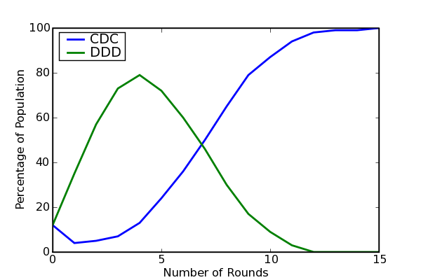
Figure 1: Evolving Strategy Frequencies on an Evolutionary Grid (P=1)
6.9
We can understand the success of the CD-C strategy that we see in Figure 1 in terms of our previous results in Table 3.
Consider two adjacent CD-C players on a grid that is otherwise
entirely populated by DD-D players.
Using the notation of Rapoport and Chammah (1965),
let the payoff matrix be represented symbolically as [[(R,R),(S,T)],[(T,S),(P,P)].
When playing a four-move game against a DD-D player,
a CD-C player receives a payoff of S+3P.
When playing a against a CD-C player,
a CD-C player receives a payoff of 4R.
Given our standard (von Neumann, radius 1) neighborhood,
a CD-C player on this grid will have three DD-D neighbors and one CD-C neighbor.
Its total payoff from a round is therefore 4R+9P+3S.
| DD-D 16P |
DD-D T+15P |
DD-D T+15P |
DD-D 16P |
| DD-D T+15P |
CD-C 4R+9P+3S |
CD-C 4R+9P+3S |
DD-D T+15P |
| DD-D 16P |
DD-D T+15P |
DD-D T+15P |
DD-D 16P |
6.10
Next, consider a DD-D player playing four-move games on the grid described above.
A DD-D player who plays a game against a CD-C player receives a payoff of T+3P.
A DD-D player who plays a game against a DD-D player receives a payoff of 4P.
So a DD-D player who has a CD-C neighbor gets a one-round payoff of T+15P,
while a DD-D player who has only DD-D neighbors gets a one-round payoff of 16P.
6.11
Now consider the implications of these payoffs in an evolutionary prisoner's dilemma.
In the literature it is fairly common to let each game run for four iterations.
For concreteness, we focus on this four-move game.
In this case, the two adjacent CD-C players get a higher payoff than their DD-D neighbors as long as 4R+3S>T+6P.
Recall the canonical prisoner's dilemma payoffs: [[(3,3),(0,5)], [(5,0),(1,1)].
This means that the highest average payoff will go to our two adjacent CD-C players.
(The two CD-C players in this case each receive a payoff of 21,
while a DD-D neighbor will receive 20.)
The neighboring DD-D players will therefore switch strategies.41
This increases the number of adjacent CD-C players.
Therefore, the “Tit-for-Tat” strategy quickly takes over the grid.
6.12
Contrary to a common impression,
our results do not mean that CD-C is the best strategy on our evolutionary grid.
Three obvious changes will affect whether DD-D or CD-D wins the evolutionary race.42
One possibility is to change the number of moves in each game.
(For example if we recalculate Table 5 for a 3-move game,
the two CD-C players each receive a payoff of 3R+6P+3S=15,
while a DD-D neighbor will receive T+11P=16.)
Greater interest attends deviations from the canonical payoff matrix we have been using.
Finally, we might alter our understanding of the evolutionary significance of the payoff.
6.13
Here we briefly explore the second and third possibilities.
To keep the discussion focused, we will change a single parameter: P.
Consider for example raising the value of P,
retaining the canonical payoffs T=5, S=0, and R=3.
Recall our isolated CD-C pair will beat their DD-D neighbors as long as 4R+9P+3S>T+15P:
that is, as long as 7/6>P.
If we raise P above this threshold,
then the DD-D neighbors will win and the CD-C pair will switch strategies.
Intuitively, if we increase the payoff for mutual defection,
we expect defection to be more likely to persist as a strategy (Rapoport and Chammah 1965).
6.14
Once we have P>7/6,
this eliminates the ability of isolated pairs to spread,
but it is still plausible that CD-C players will dominate in a given tournament.
Larger groups of CD-C players may be part of an initial distribution of players,
or may emerge as other player types vanish,
and these will achieve higher payoffs.
To make this concrete,
consider four CD-C players arranged in a square,
who are completely surrounded by DD-D players.
| DD-D 16P |
DD-D 16P |
DD-D 16P |
DD-D 16P |
DD-D 16P |
DD-D 16P |
| DD-D 16P |
DD-D 16P |
DD-D T+15P |
DD-D T+15P |
DD-D 16P |
DD-D 16P |
| DD-D 16P |
DD-D T+15P |
CD-C 8R+6P+2S |
CD-C 8R+6P+2S |
DD-D T+15P |
DD-D 16P |
| DD-D 16P |
DD-D T+15P |
CD-C 8R+6P+2S |
CD-C 8R+6P+2S |
DD-D T+15P |
DD-D 16P |
| DD-D 16P |
DD-D 16P |
DD-D T+15P |
DD-D T+15P |
DD-D 16P |
DD-D 16P |
| DD-D 16P |
DD-D 16P |
DD-D 16P |
DD-D 16P |
DD-D 16P |
DD-D 16P |
6.15
Each of the four CD-C players has two CD-C neighbors and two DD-D neighbors.
Each therefore receives a payoff of 8R+6P+2S (one round, four moves per game).
The neighboring DD-Ds each get a payoff of T+15P.
The CD-Cs have the better payoff if 8R+6P+2S>T+15P.
Again retaining T=5, R=3, and S=0,
this means that as long as 19/9>P the CD-C players will have the higher payoff.
All the DD-D neighbors will thereafter adopt CD-C strategies,
and this expansion will continue outward from the initial square.43
6.16
In more general terms, as we raise the payoff to mutual defection,
it becomes harder and harder for the CD-C strategy to win out over the DD-D strategy on our evolutionary grid.
The canonical payoff matrix makes it almost inevitable the CD-C player type will come to dominate the grid.
As we raise the value of P high enough,
it becomes almost inevitable for the DD-D player type to come to dominate the grid.
This can happen relatively soon.
Figure 2 illustrates the outcome when the simulation underlying Figure 1 is rerun
with no other changes than a new payoff matrix: [[(3,3),(0,5)],[(5,0),(P,P)]],
where P varies from its canonical value of 1 to the higher value 2.
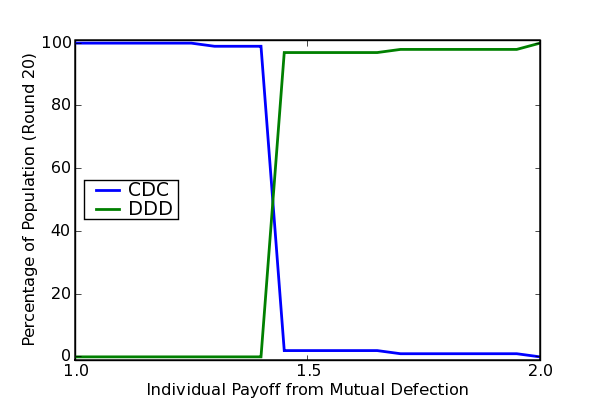
Figure 2: Strategy Persistence as Payoffs Vary
6.17
Figure 2 suggests one underappreciated way in which outcomes on an evolutionary grid can be fragile:
cardinal payoffs matter.44
Before leaving the evolutionary grid,
we briefly explore one other underappreciated way in which such simulation results can prove fragile.
So far players have evolved by imitating a top-scoring player type.
However when a player faces multiple opponents who share a playertype,
other assessments of the best playertype are plausible.
We consider a player who chooses the encountered playertype that had the highest minimum outcome:
the MaxminGridPlayer.
Since a top scoring playertype might also perform poorly against different neighbors,
top scoring playertypes will not always appear to be “best” by this maxmin criterion.
class MaxminGridPlayer(GridPlayer):
    def choose_next_type(self):
        # find playertype(s) with the highest minimum score
        best_playertypes = maxmin_playertypes(self)
        # choose randomly from these best playertypes
        self.next_playertype = random.choice(best_playertypes)
6.18
Bragt et al. (2001) show that “selection schemes” affect outcomes in an evolutionary IPD.
Here we extend this into the consideration of fitness evaluation.
This is appropriate in our IPD since strategy evolution is rooted in imitation.
We explore this possibility by introducing the MaxminGridPlayer.
This is just a GridPlayer with a new choose_next_type method,
which treats as best those encountered playertypes with the highest minimum outcome.
(Implementation details for the maxmin_playertypes function are in Appendix A.)
Again, the simplicity with which we can make this change shows how easy it
is to adapt our core game-simulation toolkit to new considerations.
Figure 3 considers the same player grid as Figure 2, with one difference:
the best strategy encountered is taken to be the one with highest minimum score.
Note that the outcomes are changed in interesting ways:
the CD-C players are squeezed out just a surely but more slowly as we increase P,
and both CD-D and DD-D playertypes are eventually able to persist.
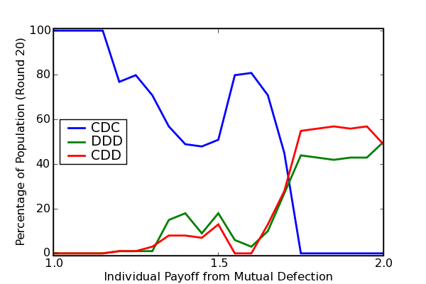
Figure 3: Strategy Persistence and Payoffs (best=maxmin)
7.1
Researchers often promote agent-based simulation (ABS) methods as a “third way” of doing social science,
distinct from both pure theory and from statistical exploration (Axelrod 1997).
One hope of ABS researchers is that unexpected but useful (for prediction or understanding) aggregate outcomes will emerge from the interactions of autonomous actors.
The evolutionary iterated prisoner's dilemma is a good illustration of the fruition of this hope:
more than two decades of computational exploration have delivered many interesting and surprising results.
Classic among these is the high fitness of the “Tit-for-Tat” player type in certain evolutionary grid environments,
which many researchers have found suggestive of the evolution of cooperation among real-world agents.
7.2
Students, teachers, and researchers naturally search for entry points to agent-based simulation.
This paper provides such an entry point.
We use the iterated prisoner's dilemma as a springboard into
agent-based simulation with the Python programming language.
This demonstrates that useful ABS models can be constructed with surprising ease
in a general purpose programming language.
Python's flexibility and object-orientation make it a powerful language for simulation,
and its syntax promotes the creation of code that is highly readable
(and therefore easily shared and maintained).
This readability does not imply verbosity:
we list in a few dozen lines
the actual source code underpinning the reported simulations.
This code is compact yet readable,
and it often bears a close resemblance to simple formal pseudocode.
7.3
A core objective of the paper is to enable students, teachers, and researchers
to begin social-science simulation projects immediately in a general purpose programming language.
The paper therefore includes a narrowly focused introduction
both to agent-based simulation and to the Python programming language.
We then introduce agent-based simulation in Python,
producing in the process an accessible basic tookit
for the simulation of two-person evolutionary games.
The reported simulations use this toolkit.
7.4
Our initial simulations introduce the iterated prisoner's dilemma
and motivate the use of agent-based models.
We demonstrate that it is possible to quickly lay bare the underpinnings of some classic results,
including the importance of topology for outcomes in evolutionary games.
We then demonstrate that one can readily extend the basic toolkit into new territory.
By altering a single entry of the payoff matrix
we demonstrate that payoff cardinality is crucial to prisoner's dilemma outcomes on an evolutionary grid.
(This provides a cautionary tale for those relying on the canonical payoffs for their simulations.)
By altering a single player method attribute,
so that the evolution of new player types is based on maximin rather than maximum outcomes,
we discover an interaction between payoff cardinality and this player attribute.
Taken as a group, the simulations in this paper provide a highly accessible but nevertheless
substantive and enabling introduction to the agent-based simulation of evolutionary games
in a general purpose programming language.
This appendix contains utilities that were used to simplify the code samples in the main text.
def mean(seq):  #simplest computation of mean
    """Return mean of values in `seq`."""
    n = len(seq)
    return sum(seq)/float(n)

def transpose(seqseq): #simple 2-dimensional transpose
    """Return transpose of `seqseq`."""
    return zip(*seqseq)

def topscore_playertypes(player):
    """Return list of best (maximum payoff) player types."""
    best_types = [player.playertype]
    best_payoff = player.get_payoff()
    for opponent in player.players_played:
        payoff = opponent.get_payoff()
        if payoff > best_payoff:
            best_payoff = payoff
            best_types = [opponent.playertype]
        elif payoff == best_payoff:
            best_types.append(opponent.playertype)
    return best_types

def maxmin_playertypes(player):
    """Return list of best (maxmin payoff) player types."""
    # initialize mapping (playertypes -> payoffs)
    pt2po = dict()
    # find minimum payoff for each encountered playertype
    pt2po[ player.playertype ] = player.get_payoff()
    for n in player.get_neighbors():
        pt, po = n.playertype, n.get_payoff()
        try:
            if pt2po[pt] > po:
                pt2po[pt] = po
        except KeyError:
            pt2po[pt] = po
    # find best playertype (max of minimum payoffs)
    maxmin = max( pt2po.itervalues() )
    best_playertypes = [ pt for pt in pt2po if pt2po[pt]==maxmin ]
    return best_playertypes

def random_pairs_of(players):
    """Return all of players as random pairs."""
    # copy player list
    players = list( players )
    # shuffle the new player list in place
    random.shuffle(players)
    # yield the shuffled players, 2 at a time
    player_iter = iter(players)
    return izip(player_iter, player_iter)

def compute_neighbors(player, grid):
    """Return neighbors of `player` on `grid`."""
    player_row, player_col = player.gridlocation
    nrows, ncols = grid.nrows, grid.ncols
    players2d = grid.players2d
    # initialize list of neighbors
    neighbors = list()
    # append all neighbors to list
    for offset in grid.neighborhood:
        dc, dr = offset      #note: x,y neighborhood
        r = (player_row + dr) % nrows
        c = (player_col + dc) % ncols
        neighbor = players2d[r][c]
        neighbors.append(neighbor)
    return neighbors

def count_player_types(players):
    """Return map (playertype -> frequency) for `players`."""
    ptype_counts = defaultdict(int) #empty dictionary, default count is 0
    for player in players:
        ptype_counts[ player.playertype ] += 1
    return ptype_counts
This appendix contains some material for teachers and students. It begins with some brief guidance on how to get up and running with Python, and how to use the code in the present paper. It then outlines a few graduated projects that can be used for further self-teaching. Finally, it suggests some resources for more advanced projects. Please note that hyperlinks in the following text point to useful resources.
Windows users can install Python in a few minutes by following the online installation instructions on the official Python website. (Others can too, but they will probably find Python is already installed.) After installation, a new user should learn to use IDLE, the cross-platform graphical programming environment included with Python. The next step is to work through sections 3, 4, and 5 of the Python Tutorial. Finally, work through section 9.3 of the Python Tutorial. You should then be ready to work with the code in the present paper.
Code presented in this paper is directly usable, once Python is installed and an interpreter is started. I will assume you installed Python and are using IDLE, as described above. Then take one of two approaches to executing the code. Approach 1: in IDLE's interpreter window, enter the code samples directly at the interpreter prompt. Approach 2: copy the code into an IDLE program window, and save as pd.py. Then use the Run menu to run the code. Start with the code first introduced, and paste subsequent code at the bottom. Whenever you need one of the utilities from Appendix A, paste it at the top of your file. (You can also find the objects and functions in the code online as the module simple_game.py.)
The official Python website contains extensive documentation, including the Python Library Reference. It is important early on to learn Python's built-in functions. (Two of the most important will be help and dir, which can provide considerable information about any object based on Python's introspection capabilities.) There is also a very active and helpful user forum, whose participants include students, teachers, hobbyists, and programming professionals.
There are many good Python books. Readers with little programming experience should find Zelle (2003) to be very helpful. Experienced programmers may want to proceed directly to the well written and helpful Python Reference Manual. In the end, the only way to learn a language is to use it. The exercises below provide a starting point.
There are several excellent graphics packages for Python. The figures in this paper are created using the Matplotlib graphics package, which has a very simple to use pylab module. After the statement import pylab, you can create a lineplot for two series x and y as simply as pylab.plot(x,y). A two-dimensional array A can be given an image representation as easily as pylab.matshow(A). (This can be used for visualizing the evolution of player types on a grid.) Matplotlib supports interactive graphics and GUI embedding.
The Matplotlib license allows royalty-free use, modification, and distribution even for commercial projects. The Matplotlib website contains binary installers, extensive documentation, and full code for a very large number of examples. There is also an active and helpful Matplotlib mailing list.
After working through these exercises, the reader should be able to implement many of the models discussed in the agent-based game simulation literature and to use these as a springboard for developing original models. Readers who wish to work on the prisoner's dilemma may find Gotts et al. (2003) to provide useful additional background and context.
 Return to Contents of this issue
© Copyright Journal of Artificial Societies and Social Simulation, [2008]