James Millington, Raúl Romero-Calcerrada, John Wainwright and George Perry (2008)

An Agent-Based Model of Mediterranean Agricultural Land-Use/Cover Change for Examining Wildfire Risk

Journal of Artificial Societies and Social Simulation vol. 11, no. 4 4
<https://www.jasss.org/11/4/4.html>

For information about citing this article, click here

Received: 30-Sep-2007    Accepted: 10-Jul-2008    Published: 31-Oct-2008

Abstract

Humans have a long history of activity in Mediterranean Basin landscapes. Spatial heterogeneity in these landscapes hinders our understanding about the impacts of changes in human activity on ecological processes, such as wildfire. The use of spatially-explicit models that simulate processes at fine scales should aid the investigation of spatial patterns at the broader, landscape scale. Here, we present an agent-based model of agricultural land-use decision-making to examine the importance of land tenure and land use on future land cover. The model considers two 'types' of land-use decision-making agent with differing perspectives; 'commercial' agents that are perfectly economically rational, and 'traditional' agents that represent part-time or 'traditional' farmers that manage their land because of its cultural, rather than economic, value. The structure of the model is described and results are presented for various scenarios of initial landscape configuration. Land-use/cover maps produced by the model are used to examine how wildfire risk changes for each scenario. Results indicate that land tenure configuration influences trajectories of land use change. However, simulations for various initial land-use configurations and compositions converge to similar states when land-tenure structure is held constant. For the scenarios considered, mean wildfire risk increases relative to the observed landscape. Increases in wildfire risk are not spatially uniform however, varying according to the composition and configuration of land use types. These unexpected spatial variations in wildfire risk highlight the advantages of using a spatially-explicit agent-based model of land use/cover change.

Keywords:

Land Use/Cover Change, Land Tenure, Wildfire, Mediterranean-Type Ecosystem, Agriculture, Spatial Heterogeneity

Introduction

1.1

Humans are the primary cause of wildfire in the landscapes of the Mediterranean Basin. For example, 95% of all wildfires in Spain are the result of human activity (Moreno et al. 1998). Changes in human activity and land-use practices in these landscapes have the potential to modify the magnitude, timing and frequency of wildfires (collectively known as the wildfire regime) as a result of changes in land-cover compositions and configurations. For example, recent increases in forest land cover in the northern Mediterranean Basin have been attributed, in part, to the abandonment of traditional low-intensity agricultural practices (Mazzoleni et al. 2004). Land Use/Cover Change (LUCC) of this type is likely to increase the biomass available to burn in the landscape, potentially leading to increased wildfire sizes.

1.2

Previous models that consider the spatial interaction of vegetation dynamics (the establishment, growth and competition between plant species) and wildfire regimes have seldom considered the influence of human activity on these interactions. The few models that have considered human activity have done so by considering general scenarios of human impact, imposed exogenously (e.g., Baker 1995; Perry and Enright 2002). However, an agent-based approach provides significant advantages over scenario-based approaches. These advantages include the representation of emergent (spatial) patterns of LUCC from hypothesized behaviour and the provision of mechanisms for dynamic feedback (Wainwright 2008).

1.3

Here we present an Agent-Based Model of Land Use/Cover Change (ABM/LUCC) that is used to evaluate potential changes in wildfire risk for a Mediterranean landscape. Our ABM/LUCC simulates a traditional Spanish agricultural landscape that is undergoing social, demographic and cultural change. Specifically, agricultural location theory is complemented by the elicitation of agent behaviour specific to the study area from local agricultural actors, to produce an agent-based model of agricultural decision-making. We then use maps of land-cover composition and configuration that emerge from the interaction of agents' land-use decision-making to assess potential impacts on wildfire risk.

Modelling agricultural land-use patterns

2.1

Classical agricultural location theory was developed to explain the spatial location of agricultural land-uses and practices. The von Thünen (1826) model assumes that an individual has perfect knowledge of prices and costs, perfect economic rationality on the part of producers (i.e., the product that provides greatest profit is always chosen), and homogeneity of all other environmental factors (including soil fertility, labour availability etc.). Using this model, von Thünen showed that generalised land uses with varying economic yields and transport costs form concentric rings around a single central market. Chisholm (1962) introduced von Thünen's theory into rural geography to explain spatial patterns of agricultural land use by examining relative and absolute locations and distances of a variety of production entities at multiple organisational levels and spatial scales. Many critics have noted the importance of Chisholm's work (Cliff et al. 1997), but also highlight the incompleteness of such a spatially-dependent theoretical framework (e.g. Moran 1994; Munton 1994). Munton (1994) highlighted that there are many other important factors alongside transport costs associated with the distance of a location to a market in determining the spatial allocation of agricultural land-uses. These factors include trade agreements, agricultural subsidies, and land-tenure history, among others. Harvey (1966, p. 370) summarised, "the only way we can understand regional variations in agriculture will thus be through an understanding of decision-making processes; and decisions are never simply economic ones". It is from such criticisms that recent agent-based approaches have emerged as a means of considering the influence of individual agents' behaviour on LUCC.

2.2

Several recent reviews of the use of ABM/LUCC highlight the increasing interest in their application (Parker et al. 2003; Bousquet and Le Page 2004). These models typically represent feedbacks between decision-making agents and a cellular model of the physical landscape (Parker et al. 2003). This model framework provides several representational improvements over classical agricultural location approaches. First, the approach is process-based and considers the behaviour of the actors making the decisions that influence land-use patterns. Second, by considering agents' actions spatially-explicitly, ABM/LUCC allow the dynamic representation of interactions between socio-economic and biophysical processes. Consequently, agents' behaviour, and in turn the spatial distribution of land uses, can be interpreted in a spatially-explicit manner across a range of scales (depending on what actor the agent represents and the grain at which the landscape is represented). The spatially-explicit and agent-based characteristics of ABM/LUCC mean that the socio-economic and biophysical processes and structures being represented can be examined at their appropriate scales. Thus, this model framework allows an improved representation of the impacts of heterogeneous spatial decision-making conditions on individual land holders' decisions.

2.3

Many studies using ABM/LUCC have focused on conversion of virgin tropical forest to other non-forest land uses and covers (e.g. Evans et al. 2001; Deadman et al. 2004; Huigen 2004; Manson 2005). In contrast, agriculture has a long history in the Mediterranean Basin (Grove and Rackham 2001; Wainwright and Thornes 2004), and contemporary processes of LUCC are generally not the result of the conversion of forest or woodland to agricultural uses.

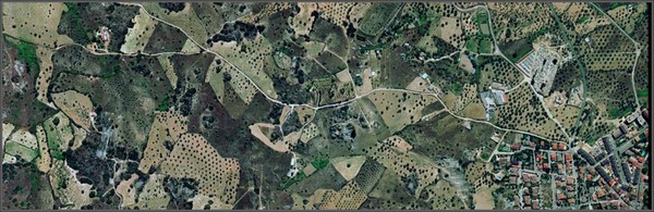
Figure 1. The fragmented and heterogeneous spatial structure of a traditional Mediterranean agricultural landscape. The aerial photograph from the study area spans approximately 1.6 km (1 mile) and contains numerous land-use and cover types including pasture, crops and urban areas.

2.4

In this paper we consider LUCC in a traditional Mediterranean agricultural landscape, EU Special Protection Area number 56 (SPA 56) 'Encinares del río Alberche y Cofio', in central Spain. Fragmented land tenure in SPA 56 is a result of repeated land division between family heirs over many generations. Furthermore, central Spain's semi-arid climate (mean annual rainfall is 400 – 800 mm depending on altitude), high intra- and inter-annual rainfall variability, irregular and often sharp relief, variable soil quality and high mean altitude (over 700 m ASL) make for adverse farming conditions in many areas. These conditions have led to a "mosaic of farming landscapes with an uneven production capacity and a complex social and environmental composition" (Peco et al. 2000 p.146). This spatial mosaic of agricultural land-use results, in turn, in a spatially heterogeneous land cover (Figure 1) with consequences for spatial ecological processes such as wildfire and vegetation seed dispersal. Social and economic trends have driven recent abandonment of agricultural land in SPA 56 (Romero-Calcerrada and Perry 2004; Millington et al. 2007), leading to increased wildfire risk (Millington 2005). Improved understanding of the consequences of agricultural land-use decision-making on land-use and land-cover patterns will aid wildfire-management operations. In particular, we use the model presented here to investigate how scenarios of different initial land-use and land-tenure influence trajectories of LUCC and the subsequent consequences for wildfire risk. Other Agent-Based Models (ABMs) have been developed to examine agricultural decision-making, policy and change in European landscapes (Balmann 1997; Mathevet et al. 2003; Happe et al. 2006). However, we believe that our model is the first ABM to consider contemporary agricultural land-use decision-making and wildfire in the Mediterranean Basin.

Model Structure

3.1

To develop an appropriate model structure and parameterisation, five semi-structured interviews were undertaken in November 2005 with local stakeholders from within SPA 56, each of whom had knowledge of specific regions of the study area due to their occupation and, in most cases, place of residence. Interviewing the actors represented in an ABM is a useful way of developing system understanding to ensure agent behaviour is representative of actual behavioural patterns (Matthews and Selman 2006). Interviewees were selected from a range of institutional contexts, and included private individual land owners, a local agricultural co-operative official and a local council (ayuntamiento) official. Interviewees were specifically asked about local agricultural land use and associated income sources. Attitudes toward recent LUCC, and the understood causes, were also explored (see Millington 2007). Responses from these interviews were used to specify the agricultural land-use decision-making process of local stakeholders. Specifically, two distinctively different 'types' of farmer emerged from the interviews, each representing different worldviews: commercially-minded ('commercial') and traditionally-minded ('traditional') farmers. These two types of agent take different land-use decision-making approaches to establish whether an area of land (i.e., a pixel) will be in one of three possible land uses: crops (vineyards, orchards), pasture (goats and sheep) or non-agricultural land. Agents perceive the landscape as a grid of finite land units (i.e., pixels) on a seasonal basis (i.e., four time-steps per year). Pixels with orthogonal neighbours owned by the same agent are considered to be pixel 'clusters' (i.e., farmers' fields). The status of each agent (age, wealth, etc.) is monitored at each time-step (Figure 2).

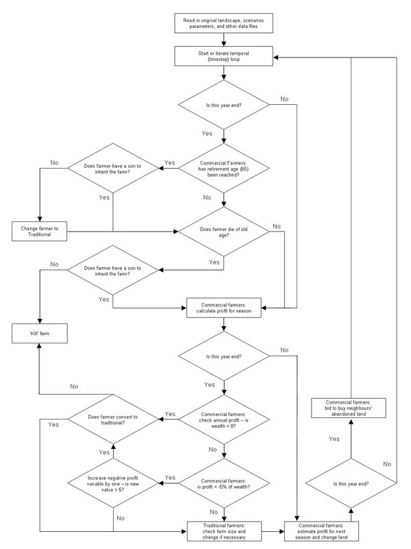
Figure 2. Procedure of the agent-based model of land-use decision-making. During each time-step seasonal functions are executed; annual functions are executed every fourth time-step (i.e., four seasons are simulated per year).

Rationale for Farmer Types

3.2

It became clear during interviews with local farmers and farming officials that the representation of actors as perfectly economically rational agents would not adequately represent all farmers in the landscape. There is a clear distinction between: (i) commercial farms that operate in an economically rational, profit-maximising manner, and (ii) those that operate on a part-time basis or merely to maintain traditional agricultural practices and landscape aesthetics. One local vintner in SPA 56 suggested:

"Whoever has a vineyard nowadays is like a gardener... they like to keep it, even if they lose money. They maintain vineyards because they have done it all their life and they like it, even having to pay for it. If owners were looking for profitability there would be not a single vineyard... People here grow wine because of a matter of feeling, love for the land..."

3.3

Thus, at least some land owners maintain their farm as a 'hobby' for cultural reasons with little regard for its financial rewards. The economically-rational agent is not an appropriate representation of these 'traditional' farmers. Furthermore, many farms across SPA 56 are run to provide supplementary household income. For example, in one area a farmer stated that of the 80 livestock farmers in the area only 20 made their living solely from farming. The remainder make their primary income from alternate sources (light industry or building services nearby) but still keep some land and livestock active:

"Part-time workers? Yes, most of them... Here there are only retired people and their children, who work somewhere else, and help their retired parents with the labouring. There is no way to live on wine production."

3.4

This part-time work must be represented by the behaviour of agents of the model. In general, we might say that these traditional and part-time farmers are less concerned with the economic state of the market, and their activities will be relatively insensitive to changes in it. In contrast, those farmers whose farm is their sole source of income treat their land as a commercial enterprise:

"There are some young farmers, 5 or 6 of whom are less than 25 years old, that are making important investments. If someone wants to live from livestock farming, they need to have an entrepreneurial vision, a business mentality, like in any company."

Such farmers will adopt those land-use and farming practices that maximise their income. Different behaviours (i.e., model rules) are therefore required to characterise 'commercial' versus 'traditional' agents (Table 1). Attributes and decision-making rules common to both agent types are now described (see Table 2 for list of all attributes and parameters). Subsequently, attributes and rules unique to each agent type are discussed in detail.

Table 1: Comparison of attributes of 'traditional' and 'commercial' agents. Attributes were derived after interviews with local actors within the study area.
Attribute	Traditional Agent	Commercial Agent
Commitment	'Part-time' or 'Hobby' farmer	'Full-time' businessman
Age	Any, greater than 19 years	Maximum 65 years (retirement age)
Land Exchange	Will not exchange land	Will buy/sell land to achieve profit
Land Uses	Maintains land in 'traditional' uses	Whatever land use maximises profit
Financial Attitude	Profit is not primary determinant of behaviour	Aims to maximise profit

Table 2: Attributes and parameters considered in the model. Attributes and parameters are presented for agents, pixels, farms, and those that are universal within the model. Units CU are arbitrary 'Currency Units'.
Name	Unit	Range of Values	Description
Agent
age	Years	20 – 100	Agent's age
perspective	-	Commercial, Traditional	Agent worldview, determining behaviour
personal_choice	-	0 – 1	Propensity of an agent to become a 'commercial' farmer
wealth	CU	0 – ∞	Agent's total accumulated value
profit	CU	0 – ∞	Farm profit for this season
max_bid	CU	0 – ∞	Maximum bid an agent will offer to buy a pixel of land
poor_profit	CU	0 – Length of model replicate	Number of years that annual profit has been below the poor_profit threshold
est_profit	CU	-∞ – ∞	Agent's estimated profit for the next year
ann_profit	CU	-∞ – ∞	Total farm profit for the current year
mf_size	Pixels	0 – Area of landscape	Number of pixels agent can manage before incurring farmCost on additional pixels (age dependent)
est_valueC	CU	-∞ – ∞	Estimated valueC for the next year
est_valueP	CU	-∞ – ∞	Estimated valueP for the next year
est_costC	CU	-∞ – ∞	Estimated costC for the next year
est_costP	CU	-∞ – ∞	Estimated costP for the next year
est_farmCost	CU	-∞ – ∞	Estimated farmCost for the next year
prev_est_valueC	CU	-∞ – ∞	Estimated valueC for the last year
prev_est_valueP	CU	-∞ – ∞	Estimated valueP for the last year
prev_est_costC	CU	-∞ – ∞	Estimated costC for the last year
prev_est_costP	CU	-∞ – ∞	Estimated costP for the last year
prev_est_farmCost	CU	-∞ – ∞	Estimated farmCost for the last year
Pixel
frag_value	-	0 – 1	Fragmentation value indicating relative size and proximity of pixel to the rest of the farm
lcap	-	0 – 2	Land capability measure, higher values are more suitable for agricultural uses
state	-	Crops, Pasture, Non-Agricultural	Land use pixel is currently in
t_in_state	Years	0 – Length of model replicate	Duration pixel has remain in its current state
set_price	CU	0 – 10	CU agent is willing to sell the pixel for
road_dist	Pixels	0 – lsp_max	Distance to the nearest road
prop_farm	-	0 – 1	Proportion of farm that the pixel cluster (field) in which the pixel lies composes
Farm
max_dist	Pixels	0 – lsp_max	Greatest distance between two pixels owned by the same agent
Universal
propT	-	0 – 1	Proportion of agents in the landscape with a 'traditional' perspective
propC	-	0 – 1	Proportion of agents in the landscape with a 'commercial' perspective
valueC	CU	0 – 10	CU accrued from one pixel of crops for one season
valueP	CU	0 – 10	CU accrued from one pixel of pasture for one season
costC	CU	0 – 10	Cost of maintaining one pixel of crops for one season
costP	CU	0 – 10	Cost of maintaining one pixel of pasture for one season
farmCost	CU	0 – 10	Cost incurred per pixel in farms greater than max_farm_size or mf_size
convC	CU	0 – 1	Cost to convert a pixel from crops to pasture
convP	CU	0 – 1	Cost to convert a pixel from pasture to crops
convNA	CU	0 – 1	Cost to convert a pixel from non-agricultural to pasture or crops
lsp_max	Pixels		Maximum distance possible across the landscape
poor_years	Years	0 – Length of model replicate	Number of years of profit less than or equal to loss_resilience that an agent will sustain before retiring
loss_resilience	%	0 – 100	Profit threshold used to count poor_years
current_market_price	CU	0 – ∞	mean_tot_pixel_profit _ 40
max_farm_size	Pixels	0 – Area of the landscape	Number of pixels agent can manage before incurring farmCost on additional pixels
mean_tot_pixel_profit	CU	-∞ – ∞	Mean pixel profit for the season across all pixels owned by commercial agents

Common Agent Attributes

3.5

Each agent owns a farm, composed of a number of pixels which may be in any one of three land-uses in a single time-step. Agents have an explicit age (measured in years, one year is equal to four time-steps). The probability that an agent dies in a given year is based upon human life-tables that specify the probability of mortality of an individual given their age and country of residence (HLTD 2002). A random uniform deviate in the interval [0,1] is generated and if less than the probability specified for the agent's age, the agent is deemed to have died during this year. Upon death there is a probability that an agent will have an heir to inherit the farm and continue its maintenance; the calculation of this probability is dependent upon the type of agent (see below).

Commercial Agent Attributes

3.6

If a commercial agent dies there is an heir to inherit the farm when the following statement is true:

IF (U[0,1] < (propC + personal_choice) )

(S1)

where U[0,1] is a uniform random deviate in the interval [0,1], propC is the proportion of agents in the landscape that are commercial, and personal_choice is a parameter added to ensure that when there are no other commercial agents in the landscape there is still a chance that an heir will want to continue the business. Thus, the personal_choice parameter accounts for the personal choice of the heir and the parent's individual influence over the heir's attitudes (which are likely to be just as, if not more, important than the proportion of the local community that has the 'commercial worldview'). This value may be positive (the heir is inclined to continue the business) or negative (the heir is disinclined to continue the business). The probability of inheritance considers the proportion of commercial agents in the landscape as this is likely to be an important factor in determining whether an heir wants to continue their parent's business. If an heir inherits the farm, a new personal_choice value is set as ±10% of their parent's. The heir's age is randomly set to a value between 20 and 40, ensuring that the value is less than the dying agent's age minus 20 (assuming that farmers do not have children before the age of 20). However, if the agent is younger than 40 it is assumed that either they do not have an heir, or if they do that the heir is not old enough to assume the ownership of the farm. If there is no heir, ownership of all pixels is released (i.e., enter an un-owned state) and the farm is assumed to be abandoned.

3.7

As an alternative to bequeathing the farm to an heir at death, commercial agents may chose to retire. If the commercial agent has reached retirement age (65 years) a check is made to establish if the agent has an heir in the same manner as above (S1). If there is no heir, the agent adopts the traditional perspective. This transition is made because it is assumed that having farmed their land for all of their life, a farmer is unlikely to want to simply give up their land for nothing (a sentiment that interviews suggested to be strong). Commercial agents' land-use decisions are based on several factors related to profitability: market conditions, land-tenure fragmentation, transport costs and land productivity. Crop and pasture yields are not represented explicitly in the model and so real-world data for market conditions (i.e., profits and costs of production) are not used. Furthermore, economic market fluctuations (i.e., responses of prices to supplies and demand) are not modelled explicitly. Rather, hypothetical scenarios of crops and pasture 'values' and 'costs' (of production) are used to simulate landscapes situated in buoyant, depressed or other economic situations. Market values and costs, along with other parameters influencing agent behaviour, are tuned to represent 'business as usual' (baseline) market conditions (Table 3).

Table 3: Parameters for 'business as usual' model configuration. These initial conditions and parameter values specify the 'business as usual' (baseline) scenario (see Table 2 for definition of parameters). Results from this parameter set are used as the standard by which to evaluate the outcomes of the model experiments we conducted.
Parameter	Value
Agent Age	Uniformly random deviate in the interval [20, 65]
Conversion Costs	Non-Agricultural, 0.3; Pasture, 0.2, Crops, 0.1;
Land Use	SPA 56 1999 land use (3 uses, 109 patches)
Loss Resilience	-5%
Poor Years	5 years
Land Tenure	SPA 56 2005 land tenure (519 agents, 1213 patches)
Market Values	valueC = 5.0 valueP = 2.5, costC = 1.0, and costP=1.0
Personal Choice	Uniformly random deviate in the interval [-0.5, 0.5]
Perspective	Randomly assigned with equal probability

3.8

The spatial biophysical heterogeneity and land-tenure history of SPA 56 has resulted in a fragmented agricultural landscape. A farm in which land parcels are spatially contiguous with large land agglomeration will provide greater economies of scale than land owned by a agent that is composed of smaller, fragmented and spatial distributed parcels of land. Thus, commercial agents in the model consider land fragmentation when they calculate their estimated and actual profit:

Fragmentation Value = 1 - ( prop_farm / max_dist )

(1)

where prop_farm is the proportion of the total farm area composed by the pixel cluster (i.e., field) in which the pixel under consideration lies, and max_dist is the maximum distance between the pixel under consideration and another pixel owned (and in use) by the same agent. Thus, when prop_farm is large and max_dist is small, the fragmentation value of the pixel is low. This index penalises pixels in small clusters at great distances from other pixels owned by the agent. Distance to the nearest road or track is considered as a proxy for incurred transport costs. Direct distance to market is not considered as it is by von Thünen's model because there are multiple market locations for our study area. The cost of distance to the nearest road for each pixel is normalised by the maximum distance possible across the whole study area (giving a range for this value of [1/max_dist] to 1).

3.9

Pixel productivity is represented by a land capability index (Romero-Calcerrada 2000), which evaluates the potential of a pixel for agricultural uses by considering slope, soil type, erosion risk, moisture availability and frost risk. Pixels with greater land capability values have greater yields and are thus more profitable.

3.10

Considering these factors, commercial agents calculate profit and costs, at each time-step and for each pixel, for the three possible land-uses as follows:

Crops profit = (valueC × lcap) - (2 × frag_value × costC ) - (road_dist / lsp_max)	(2)
Pasture profit = (valueP × lcap) - costP - (road_dist / lsp_max) )	(3)
Abandoned cost = 0.1	(4)

3.11

In crop land areas, the greatest profit is earned by pixels with a high land capability, low fragmentation value, and low distance to the nearest road, when the value for crops is high and the cost of production is low. Pasture profit is calculated in a similar manner to crops, the difference being that the fragmentation value of the pixel is not considered. The rationale for this approach is that land for grazing does not afford much advantage by being clustered in large patches. Small areas of land may be used for grazing just as easily as large. However, the distance to the nearest road or track is important, as this will facilitate movement of livestock between areas of pasture and to the market. There is no immediate value provided by owning land in an abandoned state. However, the costs of doing so are also minimal; all land is assumed to be owned rather than rented, as is largely the case in SPA 56. As the land may become profitable in the future, and long term planning or forecasting of the state of the market is not represented in the model, the cost per abandoned pixel per season is minimal compared to the costs of active agricultural land-uses (i.e., non-abandoned pixels).

3.12

Profit is calculated annually for each pixel and summed across the commercial agent's entire farm. If the total farmed area exceeds a 'maximum single farmer area' (max_farm_size), for each pixel exceeding this area a further cost is subtracted from the total farm profit. This cost reflects the infrastructure and labour required to farm an area greater than that possible by a single farmer with no hired labour. This maximum area that can be maintained by a single farmer (and their family) not employing hired labour is set, in accordance with values suggested by interviewees, at 40,000 m² (0.04 km², 44 pixels).

3.13

During each season commercial agents estimate the next season's profit based on the land they currently own. Commercial agents' estimates of the values and costs for crops and pasture pixels for that next season are based on the values and costs of the current and previous seasons and the accuracy of the agents' estimates in the previous season. Each agent independently estimates the value of crop land for the next season by:

Est_ValueC = valueC + actual_value_diffcC + U[0,0.5] × (valueC - prev_est_valueC)

(5)

where actual_value_diffcC is the difference between the previous value of crops and the current value of crops, prev_est_valueC is the previous estimated value of crops. This method ensures agents can estimate future prices reasonably well when values and costs change slowly, but perform less well when changes are rapid.

3.14

If the land-use configuration of the land currently owned can be modified to improve profit, land-use conversions are made. A hierarchy of land-uses restricts some land-use conversions. In this hierarchy crop land is above pasture, which in turn is above abandoned land. An unlimited number of pixel conversions down the hierarchy may be made in any one season. Only one conversion up the hierarchy may be made in any one season. Conversion up the hierarchy (e.g., from abandoned to crop land) requires both time and money, and thus the rate at which these changes can be made is restricted in the model. Conversions down the hierarchy require considerably less resources and are achieved by reducing maintenance levels.

3.15

At each year's end, commercial agents assess the profitability of their farms. If annual profit is equal to, or less than, a specified proportion of their wealth (specified for all agents by the loss_resilience parameter), the 'poor profit' year counter is increased by one. After a given number of years of poor profit (specified by the poor_years parameter) a commercial agent becomes a traditional agent when the following statement is true:

IF (U[0,1] < (propT + personal_choice) OR age > 50)

(S2)

3.16

The first element of the statement is similar to the check made when an agent dies or reaches retirement age (S1). However, in this case the proportion of traditional agents in the local neighbourhood is considered as this will be a prime determinant on whether the commercial agent is susceptible to the 'traditional worldview' and wants to continue to farm, despite it not being their primary income. The second statement checks the age of the agent. If the agent is 50 or older they automatically become a traditional agent. This switch in perspective is based on the assumption that a younger farmer will want to move onto another job because they still have 'time on their side' to start a new career. If the farmer is older than 50, it is assumed that they will be less inclined (or skilled) to endeavour to find a new full-time career and will therefore maintain the farm as a supplementary income. If both statements are false, the farm is abandoned.

3.17

At the end of each year commercial agents can bid to buy abandoned pixels contiguous to pixels they already own. All such abandoned pixels are examined to assess whether their ownership and conversion would increase the agent's profit in the next season. The neighbouring abandoned pixel that will increase profit most is then bid for. A 'conversion cost' is factored into the cost of purchasing land. This conversion cost is a product of a conversion factor for the current land use (Table 3) and the duration a pixel has been in its current state. The duration of time in current state is used because it is an indicator of: (i) biomass levels of non-agricultural lands and (ii) how 'established' an area of land is from a historical agricultural land-use perspective. The maximum bid an agent will offer is given by:

max_bid = 4 × pixel_profit × (65 – age)

(6)

where pixel_profit is the estimated increased profit it will afford (multiplied by four seasons to give profit for a year) and age is the age of agent. The second constant is included to account for the age of the farmer, as this gives a rough guide to the number of years of profit the pixel (if bought) will provide to the farmer until retirement. If the bid is larger than the asking price of the current owner, ownership passes to the bidding agent and land-use is changed to the most profitable state. The buying agent's wealth is decreased by the asking price (not the maximum bid), and the seller's increased commensurately. If two agents bid for the same pixel, the highest bid wins (assuming it is greater than the asking price) and the maximum bid is the value that changes hands. The asking price of an agent is set as the current wealth of that agent divided by the total number of pixels owned by that agent. If the pixel is abandoned but un-owned the asking price is set to the 'current market price':

Current Market Price = 40 × mean_tot_pixel_profit

(7)

where mean_tot_pixel_profit is the mean pixel profit for the season across all pixels owned by commercial agents in the landscape. The constant gives an estimate of potential profit to be made by that pixel (in the current market state) over the next decade (i.e., 40 time-steps). If a bid is not as large as the asking price, ownership stays with the current owner and the pixel remains in the abandoned state. Whatever the result of a bid, once all agents' bids have been considered, the next season then begins.

Traditional Agent Attributes

3.18

Traditional agents follow similar rules to commercial agents regarding their succession following death but: (i) are not assumed to retire, (ii) do not consider any profit-making activities, and (iii) do not seek to buy land from neighbours. If a dying traditional agent is older than 40, the farm is inherited by a new farmer as a commercial agent when the following is true:

IF (mean_tot_pixel_profit + propC - (age / 100)) > 0

(S3)

This statement assumes that the heir will be willing to become a commercial farmer when: (i) the profit in the landscape is generally high, (ii) there are other commercial farmers in the landscape (i.e., they see that others are finding it possible to make a living from their land), and (iii) their age is low (and therefore they are assumed to be more willing to take a risk and 'give it a go'). Age is scaled to the order of mean_tot_pixel_profit and propC.

3.19

If statement S3 is false then an heir may inherit the farm as a traditional agent. There is an heir to inherit the farm when the following statement is true (similar to S1):

IF (U[0,1] < (propT + personal_choice) )

(S4)

3.20

The probability that a traditional agent has an heir is based on the proportion of traditional agents in the neighbourhood (propT), not because this is the mechanism that dictates whether there is an heir, but because this is likely to be an important factor in determining whether an heir wants to continue in the footsteps of their parent. The personal_choice parameter reflects the heir's personal attitude. Again, the heir's age is randomly set to a value between 20 and 40, ensuring that the value is less than the dying agent's age minus 20. If both checks (S3 and S4) are false the farm is abandoned.

3.21

Just as commercial agents consider a threshold area (max_farm_size) greater than which they must pay for extra maintenance costs (for hiring labour etc.), traditional agents consider a maximum farm size beyond which they cannot maintain the land. If total farm size is larger than this maximum size, the appropriate number of pixels (with the lowest land capability values of pixels at the edges of clusters in the farm) is abandoned. This maximum farm size decreases with age once the agent reaches retirement age (65 years), representing their decreasing ability to maintain land (despite potential help from relatives). This rate is given by:

mf_size = max_farm_size × exp((65 – age)/wt))

(8)

where mf_size is the maximum farm size of the retired agent, age is the age of the agent in question, and wt is a shape parameter (default value = 8, chosen in rough accordance with interviewees' understanding). Thus, the area of land a farmer is able to maintain is assumed to decrease exponentially with age after retirement.

Implementation

3.22

The ABM/LUCC was originally developed in NetLogo (Wilensky 2005) then recoded into C++ (both versions of the model are available online at http://www.landscapemodelling.net/JASSS08.html). Although the NetLogo modelling environment is very useful for developing agent-based models thanks to its simple syntax and visual output, recoding in C++ reduced execution time considerably. We use the ABM/LUCC in this paper to examine the effects of initial land-tenure and land-use composition and configuration on LUCC. Subsequently, we use the land cover maps produced to examine wildfire risk. A subset of the original SPA 56 study area data (Millington et al. 2007), containing 519 agents on a grid measuring 101 × 101 pixels (i.e., 9.2 km²), is considered for these model analyses. The effects of land use and land tenure are examined using random maps of the same dimensions. The ABM/LUCC considers three land use types; crops, pasture and non-agricultural. We consider two state variables to examine the model: (i) proportion of the land used for crops and (ii) proportion of the land used for pasture. These are the two main state variables that agents make decisions about. Measures of landscape pattern, including number of land use patches, mean patch area and a landscape contagion index, are also examined. Anonymous land-tenure maps are from the Ministerio de Hacienda (2005), Madrid. Agent attributes are generated randomly. Agents are randomly assigned an age between 20 and 65, and perspective (traditional or commercial) following a uniform random distribution. Agents are assigned a random wealth such that the population wealth distribution follows a power-law (with exponent = -1.5).

3.23

To examine the effects of land-tenure and land-use configuration, maps with random land-use and land-tenure configuration were generated using the modified random clusters method (Saura and Martinez-Millan 2000). This method specifies a percolation probability parameter P to generate landscape maps with clusters of pixels of varying (uniformly randomly distributed) size. As P increases, the number of patches in the landscape decreases and mean and maximum patch size increase. The probability that a cluster spanning the entire landscape is generated approaches a value of one at the critical percolation threshold P_c ≈ 0.59 (Saura and Martinez-Millan 2000). Random land-tenure maps were initially generated for P = 0.20, P = 0.40, P = 0.45, P = 0.50, P = 0.55, P = 0.60, and P = 0.80 (Figure 3), resulting in landscapes with numbers of agents and land-tenure parcels as specified in Table 4. Random land use maps were generated using the random clusters method to examine the influence of original land use configuration. Maps LU1, LU2 and LU3 (with P = 0.2, P = 0.4 and P = 0.5 respectively) were generated with similar land use proportions to SPA 56 land use in 1999. Although similar in land use composition, these random initial maps are spatially dissimilar to observed SPA 56 land use. For maps generated with clusters spanning the landscape (i.e., P > P_c), land use proportions comparable with original SPA 56 land use are not possible. Maps LU4 and LU5 were generated with total landscape proportions of ≈0.62 for pasture and crops respectively (with P = 0.6) and maps LU6 and LU7 were composed entirely of pasture and crops respectively (landscape proportion = 1.0).

3.24

Wildfire risk is estimated for final land-use maps using the semi-quantitative method described by Millington (2005). This approach considers factors governing both wildfire ignition (distance to roads, vegetation type and solar insolation) and wildfire spread (spatial configuration of vegetation, vegetation type, topography and human management treatments). Notably, the risk model uses the contiguity landscape pattern metric (McGarigal et al. 2002) to account for the impacts of spatial configuration on the percolation of fire through the landscape. Each variable is assigned a risk score according to its relative influence on fire ignition and subsequent spread. These scores are then weighted and summed to produce a wildfire risk score for each pixel in the landscape. The risk scores indicate the risk of that pixel burning relative to other pixels in the landscape, and also allow a comparison of risk between land cover maps of the same landscape.

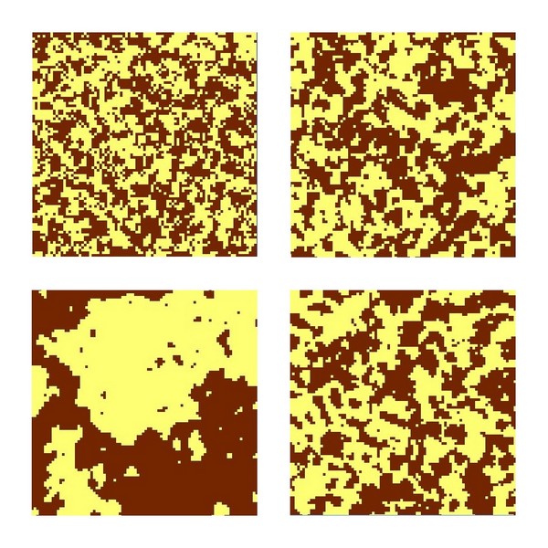
Figure 3. Examples of random maps generated with varying percolation probability parameter P. Clockwise from top left, maps are generated with P = 0.2, P = 0.4, P = 0.6 and P = 0.8. The two colours represent two different (hypothetical) land covers.

Table 4: Parameter values for ABM/LUCC testing. Parameter values were chosen to span the parameter space of the model. This allowed us to examine the range of possible model states and investigate important parameters and input data.
Scenario	Variable	Distribution of Values
LU1	Land use	P = 0.2 (SPA land-tenure, 509 LU patches)
LU2	Land use	P = 0.4 (SPA land-tenure, 291 LU patches)
LU3	Land use	P = 0.5 (SPA land-tenure, 198 LU patches)
LU4	Land use	P = 0.6 (SPA land-tenure, 94 LU patches, predominantly pasture)
LU5	Land use	P = 0.6 (SPA land-tenure, 83 LU patches, predominantly crops)
LU6	Land use	P = 0.8 (SPA land-tenure, 1 pasture patch)
LU7	Land use	P = 0.8 (SPA land-tenure, 1 crops patch)
LT1	Land tenure	P = 0.20 (511 Agents, 2653 LT patches)
LT2	Land tenure	P = 0.40 (478 Agents, 1297 LT patches)
LT3	Land tenure	P = 0.45 (442 Agents, 1005 LT patches)
LT4	Land tenure	P = 0.50 (404 Agents, 791 LT patches)
LT5	Land tenure	P = 0.55 (313 Agents, 480 LT patches)
LT6	Land tenure	P = 0.60 (224 Agents, 296 LT patches)
LT7	Land tenure	P = 0.80 (19 Agents, 19 LT patches)

Results

Initial Land Tenure

4.1

Land-tenure configuration is an important determinant of land-use decision-making in the model. Obvious differences in land-use abundance are evident across the range of possible land-tenure structures (Figure 4). There is an inverse relationship between percolation parameter P and pasture abundance (Figures 4 and 5). That is, as initial mean land-tenure parcel size increases, the simulated proportion of land devoted to pasture decreases. Model replicates highlight a large decrease in pasture abundance between random initial land-tenure maps with P = 0.55 and P = 0.60 (LT5 and LT6 respectively, Figure 4). This decrease is commensurate with P becoming greater than P_c, and is related to the maximum farm size rule.

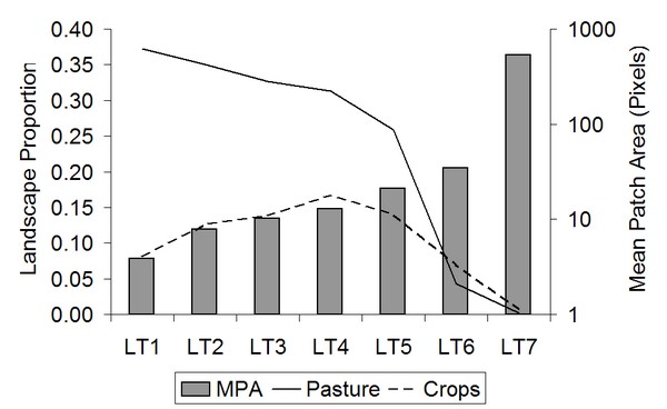
Figure 4. Landscape land-use proportions and mean land-use patch area for random land-tenure maps. An inverse relationship between abundance of pasture (solid line) and mean patch area (bars) is evident. Abundance of crops (dashed line) peaks for median mean patch area. Scenarios are specified in Table 4

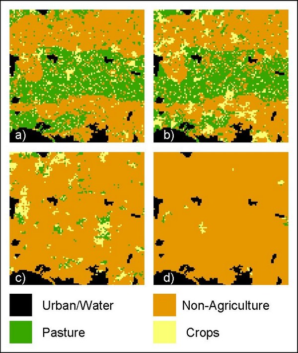
Figure 5. Land-use maps from land-tenure scenarios. a) LT1, b) LT2, c) LT6 and d) LT7 As initial mean land-tenure parcel size increases, land area devoted to pasture decreases commensurate with increases in non-agricultural land uses.

Table 5: Agricultural landscape structure characteristics for land-tenure maps. Also presented are final agricultural land-use proportions for corresponding model replicates. Land-tenure maps with p ≥ 0.60 result in landscapes with very low agricultural land-use due to the large size of patches and farms
	Initial Land Tenure			Final Agricultural* Land Use
Scenario	Agent Parcels¶	MPA‡	Small Farms†	Landscape Proportion	Number of Patches
Baseline	2.34	8.41	1.00	0.44	64
LT1	5.18	3.85	1.00	0.45	484
LT2	2.78	7.87	0.96	0.48	452
LT3	2.27	10.15	0.87	0.47	444
LT4	1.96	12.90	0.76	0.48	359
LT5	1.53	21.25	0.43	0.40	310
LT6	1.32	34.46	0.21	0.11	199
LT7	1.00	536.89	0.01	0.01	20

^¶Mean number of parcels per agent
^‡Mean parcel area (pixels)
^†Farms with size < max_farm_size (as proportion of landscape)
^*Crops plus pasture

4.2

Initial mean number of land-cover patches per agent and mean land-tenure parcel area are comparable to the observed SPA land-tenure (in 2005) and to scenario LT2 (Table 5). The most area in agricultural land-use after a 50-year model replicate is 48% of the landscape (scenario LT2), while agricultural land-use accounted for 41% of SPA 56 in 1999 (and 44% after a 50-year model replicate using original SPA 56 land-tenure, Table 5). However, the model produces land use maps that are patchier relative to initial land-use and original SPA 56 maps (except for LT7, Table 5).

Initial Land-Use

4.3

Land-use scenarios tend toward a similar final land-use configuration but differ in their land-use compositions (Figure 6). Scenarios LU1, LU2 and LU3 differ least from results for the model initiated with the original SPA 56 land-use map. By contrast, scenarios LU4 – LU7 are driven by initial dominant land-uses and result in markedly different land-use compositions.

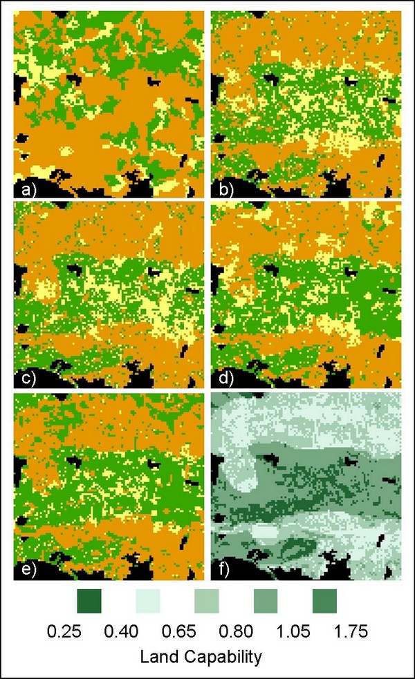
Figure 6. Land-use maps from land-use scenarios. a) Original SPA land-use, b) LU1, c) LU2, d) LU5, e) LU7 and f) land capability. Key for land-use maps as in Figure 5. Simulated maps for model replicates of land-use scenarios (b – e) converge toward a similar configuration, related to land capability patterns (f). This land-use relationship is stronger between model maps than with the empirical map (a)

4.4

Simulated land-use maps are more fragmented than their initial land-use configuration (except for LU6 and LU7) and are characterised by more patches and lower contagion values (Table 6). Contagion is a measure, from 0 (i.e., each pixel is a different patch type) to 100 (i.e., landscape is a single patch) of the spatial aggregation of patch types in the landscape (McGarigal et al. 2002). Thus, more patches and lower contagion indicates a more spatially fragmented ('patchy') landscape than one with fewer patches and high contagion values. Simulated map configurations are similar to the spatial configuration of land capability (Figure 6). Land capability values are significantly different between land uses (Kruskal-Wallis tests for scenarios LU1 – LU7 all with p < 0.001). A pixel-by-pixel comparison of simulated and initial land-use maps shows that resultant maps are more similar to one another than to their initial configuration.

Table 6: Spatial metrics of land-use pattern for land-use scenarios. Spatial metrics examined are the number of patches (NP) and contagion (CONTAG). Greater numbers of patches and smaller contagion values indicate a more fragmented ('patchy') landscape. This is the case for simulation results compared with initial land-use configuration in each case. Scenarios are specified in Table 4
	Initial			Final
Scenario	NP	CONTAG		NP	CONTAG
Baseline	79	33.0		514	38.8
LU1	509	22.5		552	20.8
LU2	291	30.3		541	24.1
LU3	198	35.4		499	21.9
LU4	130	43.0		403	24.3
LU5	126	43.5		446	22.1
LU6	1	100.0		380	30.8
LU7	1	100.0		359	23.7

Consequences for Wildfire Risk

4.5

For all scenarios (except LU7), mean and standard deviations of wildfire risk for maps produced by land-tenure and land-use scenarios are greater than observed SPA56 wildfire risk in 1999 (Table 7). Mean wildfire risk values are similar between scenario results, highlighting the similarity of land-use configurations resulting from the scenarios simulated. However, there is a marked difference in the locations of pixels with high and low risk of burning between land-tenure and land-use scenarios (Figures 7 and 8).

Table 7: Estimated wildfire risk. Mean, standard deviation, minimum and maximum values are reported for maps from each scenario and from the original, observed landscape (SPA). Generally, mean risk is greater for landscapes resulting from model scenarios. However, maximum values and standard deviations are also greater, indicating that a few very high risk locations are driving these increases
	Wildfire Risk
Scenario	Mean	St. Dev.	Min	Max
SPA	108.2	31.2	31.6	203.8
LU1	121.5	44.4	20.0	240.3
LU2	118.1	42.6	16.0	234.4
LU3	119.6	43.4	20.0	238.4
LU4	118.4	42.1	23.3	234.6
LU5	128.6	43.3	18.1	242.6
LU6	158.7	36.1	16.9	248.5
LU7	172.7	21.9	44.3	252.4
LT1	108.3	42.7	15.0	228.6
LT2	120.6	43.6	22.1	239.3
LT3	120.5	43.3	20.0	238.4
LT4	115.9	41.9	20.0	240.3
LT5	115.7	42.7	20.0	239.8
LT6	113.4	43.9	20.0	240.4
LT7	83.9	27.7	20.0	192.4

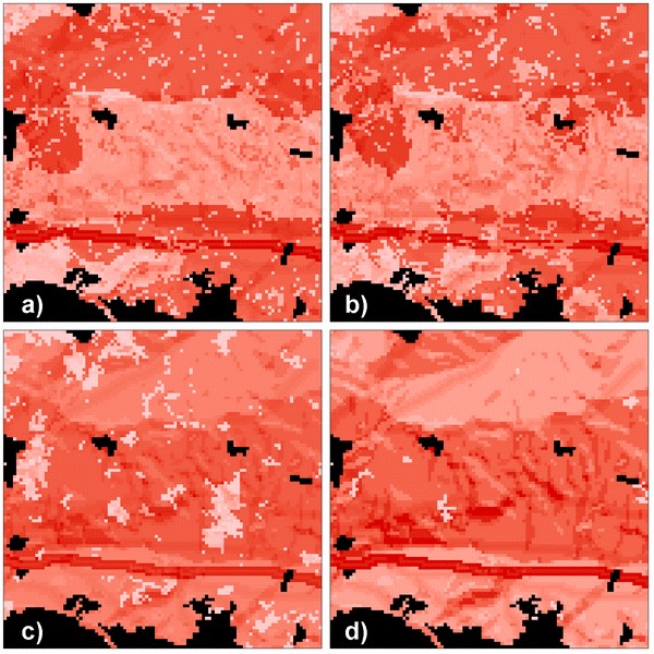
Figure 7. Wildfire risk maps from land-tenure scenarios. a) LT1, b) LT2, c) LT6 and d) LT7. Scenarios resulting in greater agricultural land use (a and b) produce different wildfire risk patterns than those with lesser agricultural land use (c and d). Risk values are relative for each map – darker colours indicate greater risk. The line of high-risk running roughly horizontally across all maps is due to a road running through the landscape.

4.6

Simulated maps for land-tenure scenarios with lower values of P (Figures 7a and 7b) have greater wildfire risk in the north of the study area relative to the central region (north of the road running east to west as indicated by highest risk values). This spatial pattern is also the case for land-use scenarios (Figures 8a and 8b). In contrast, wildfire risk for the original SPA land use map (Figure 8a) and simulated maps for land tenure scenarios LT6 and LT7 (with greatest value of P, Figures 7c and 7d) have greater risk in the central region than the northern. These differences highlight that the context in which LUCC decisions are made has consequences for both the magnitude and spatial distribution of wildfire risk.

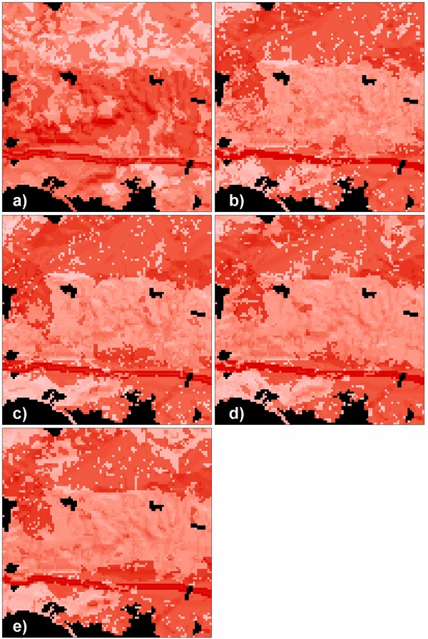
Figure 8. Wildfire risk maps from land-use scenarios. a) Original SPA land use, b) LU1, c) LU2, d) LU5 and e) LU7. Maps for b) to d) have similar spatial patterns, reflecting the convergence of land-use scenarios to similar land-cover configurations (see Figure 6). Risk values are relative for each map – darker colours indicate greater risk. The line of high-risk running roughly horizontally across all maps is due to a road running through the landscape.

Discussion

5.1

The ABM/LUCC presented here synthesises knowledge from several sources, including established formal agricultural location theory, other agent-based modelling projects, and the knowledge of local actors within the study area. Given the current limited understanding of the relationship between land-tenure and LUCC in the Mediterranean Basin, and in the face of limited empirical data, the modelling undertaken here was heuristic in nature rather than predictive (as others have suggested is currently most appropriate, Matthews and Selman 2006). Methods for analysing heuristic models are less established than for explicitly predictive models but approaches that rely less on formal predictive accuracy are emerging (Perry and Millington 2008).

5.2

Model results indicate that agricultural land-use decreases as initial mean land-tenure parcel size increases (Figure 4). As the rules specified in the model favour crops on larger land-tenure parcels, the observed decrease in pasture abundance might be expected to be due to the replacement of pasture by crops. However, the proportion of the landscape used for crops peaks at an initial random land-tenure landscape of P = 0.50 (Figure 4). For P ≤ 0.55 a dominance of pasture indicates this land use is the most profitable for farmers. For P ≥ 0.60, land-tenure parcels are so large that the maximum farm size rule becomes an influence on land-use decision-making. Thus, fewer farmers farming a subset of larger farms results in decreased land-use (both pasture and crop land-uses, Table 5 and Figure 5). Comparison of these land-tenure scenario results with the land-tenure configuration of SPA 56 in 2005 indicates that the actual land-tenure configuration is near that for which most land can feasibly be used (given model assumptions of traditional family farms, little mechanisation etc.). The current land-tenure configuration of SPA 56 is very similar to the initial land-tenure configuration of the model scenario resulting in the greatest area of agricultural land use (LT2).

5.3

At the outset of this paper we discussed the potential importance of individual actor circumstances and spatial heterogeneity on agricultural land-use decision-making. Our simulated landscapes tended to converge toward similar landscape states, in terms of land-use configuration and composition, regardless of initial land-tenure or land-use configuration. Particularly, we find statistically significant differences between land-use land-capability values for model results, but not for observed values. This suggests that land capability plays a more important role in land-use decision-making in the model than is in evidence in SPA 56. These findings question the importance of space and actor context in agricultural decision-making as it is represented in the model. Identifying cases in which spatial pattern is critical for understanding LUCC decision-making, versus those in which it is not, is likely to reveal important differences between landscape function. In turn, these differences will result in different trajectories of change.

5.4

Further investigation into the relative importance of land capability versus spatial patterns of other factors (such as land tenure) for LUCC in the SPA 56 landscape may be pursued by engaging local stakeholders. Evaluating model structure and results by returning to consult with local stakeholders that were interviewed initially (as described above), creating an iterative model development process, has been advocated for agent-based modelling projects (Parker et al. 2003). Although this process is unlikely to directly address the model output issues discussed above (i.e., patchiness of maps produced by the model, importance of land capability), it does offer a way to identify potential model improvements that are not apparent from comparing model output with empirical data. An initial stakeholder evaluation of the model presented in this paper found that stakeholders generally accepted that the model structure was representative of decision-making processes and that outputs matched anticipated future change reasonably well (Millington 2007). However, shortcomings in model structure were highlighted, most importantly the lack of representation of urban change and an over-emphasis on the spatial aspect of agricultural decision-making (Millington 2007). Recently, Romero-Calcerrada et al. (2008) found that human access to the landscape is an important predictor of wildfire ignition. This finding reiterates the importance of representing urban change in the model, particularly if the model is to be used to examine impacts of human-driven landscape change on wildfire regimes.

5.5

We used our ABM/LUCC to examine the potential impacts of various scenarios of initial landscape land-use and land-tenure configuration on wildfire risk. Mean wildfire risk for simulated land-use maps was generally greater than for the SPA 56 landscape observed in 1999. This result seems counter-intuitive given that the proportion of agricultural land-use increased for many scenarios (Table 5), as did land-cover fragmentation (Table 6). This is counter-intuitive because the scoring and weighting used in the wildfire risk calculations (Millington 2005) assumes increased patchiness of less flammable land covers would result in decreased wildfire spread and ignition, and therefore decreased wildfire risk. However, the greater mean values observed for simulated maps are driven by greater maximum risk values of individual pixels in the simulated landscapes, as reflected by greater standard deviations. Furthermore, the spatial distribution of risk varies between simulation results according to agricultural land area. For scenarios that result in greater agricultural land use than observed in the original SPA 56 landscape (i.e., LT 1 – LT4), wildfire risk is greater in the north of the study area compared with the central region (Figure 7). In contrast, for scenarios which result in decreased agricultural land-use (i.e., LT5 – LT7) risk is greater through the central region – a pattern similar to that observed for the original SPA 56 land-use map (Figures 7 and 8). These unexpected variations in spatial wildfire risk distribution highlight the advantages of using a spatially-explicit ABM/LUCC. Understanding spatial variation in wildfire risk due to human activity will be a vital consideration for wildfire managers in the region (Romero-Calcerrada et al. 2008). This will be important, for example, when strategically allocating wildfire fighting and mitigation resources at high-risk locations in the future.

5.6

Notwithstanding the convergence of simulated landscapes to similar land-use states, our results highlight the role of spatially-explicit models in understanding the potential consequences of LUCC. These consequences may be changes in the wildfire regime, as in this particular investigation, but may also be any one of a number of landscape ecological processes such as soil erosion or changes in endangered species habitat, both of which are issues in Mediterranean landscapes. Furthermore, the wildfire risk modelling undertaken here was static, in the sense that feedbacks in time between LUCC and wildfire occurrence were not considered. It may be the case that when other processes (such as wildfire) are incorporated dynamically into the simulated LUCC decision-making process, the spatial aspects of decision-making become much more important.

5.7

The work presented here is part of a wider modelling effort to explore the relationships between LUCC and wildfire regimes in central Spain (Romero-Calcerrada and Perry 2004; Millington 2005; Millington 2007; Millington et al. 2007; Romero-Calcerrada et al. 2008). When linked with a cellular-automata model of ecological succession and wildfire this ABM/LUCC will comprise an integrated socio-ecological simulation model of SPA 56 (Millington 2007). The integrated model will include the consideration of ignition as a result of human activity, and factors controlling wildfire spread such as slope and wildfire management treatments (e.g., fire breaks). Integrating the two types of model in this manner provides the opportunity to examine the fine scale mechanisms and interactions between human activity and wildfire regimes. If developed appropriately, the use of integrated models of this type will overcome the drawbacks of using static scenarios of human behaviour and allow a richer interpretation of human-landscape interactions (Wainwright 2008).

Acknowledgements

We are grateful to David O'Sullivan for his ideas and comments during the construction of the model. We also thank two anonymous reviewers for their comments on an earlier draft of the manuscript which help to focus our ideas and discussion. This research was initiated while the first author was on an overseas institutional visit funded by the UK Economic and Social Research Council at the School of Geography, Geology and Environmental Science, University of Auckland, New Zealand. Further support was provided by a UK ESRC/NERC Interdisciplinary Studentship (PTA-036-2003-00009).

References

BAKER, W. L. (1995). Long-Term Response of Disturbance Landscapes to Human Intervention and Global Change. Landscape Ecology 10(3): 143-159.

BALMANN, A. (1997). Farm-based modelling of regional structural change: A cellular automata approach. European Review of Agricultural Economics 24(1): 85-108.

BOUSQUET, F. and C. Le Page (2004). Multi-agent simulations and ecosystem management: a review. Ecological Modelling 176(3-4): 313-332.

CHISHOLM, M. (1962). Rural Settlement and Land Use: An Essay in Location. London, Hutchison University Library.

CLIFF, A. D., P. Haggett and R. Martin (1997). Michael Chisholm: An appreciation. Regional Studies 31(3): 205-210.

DEADMAN, P., D. Robinson, E. Moran and E. Brondizio (2004). Colonist household decision making and land-use change in the Amazon Rainforest: an agent-based simulation. Environment and Planning B-Planning & Design 31(5): 693-709.

EVANS, T. P., A. Manire, F. de Castro, E. Brondizio and S. McCracken (2001). A dynamic model of household decision-making and parcel level landcover change in the eastern Amazon. Ecological Modelling 143(1-2): 95-113.

GROVE, A. T. and O. Rackham (2001). The nature of Mediterranean Europe: An ecological history. London, Yale University Press.

HAPPE, K., K. Kellerman and A. Balmann (2006). Agent-based analysis of agricultural policies: an illustration of the agricultural policy simulator AgriPoliS, its adaptation, and behavior. Ecology and Society 11(1): 49.

HARVEY, D. W. (1966). Theoretical Concepts and Analysis of Agricultural Land-Use Patterns in Geography. Annals of the Association of American Geographers 56(2): 361-374.

HLTD. (2002). Human Life-Table Database, Spain 1998-1999. Retrieved 25/07/2006, from http://www.lifetable.de/data/MPIDR/ESP_1998-1999.txt.

HUIGEN, M. G. A. (2004). First principles of the MameLuke multi-actor modelling framework for land use change, illustrated with a Philippine case study. Journal of Environmental Management 72(1-2): 5-21.

MANSON, S. M. (2005). Agent-based modeling and genetic programming for modeling land change in the Southern Yucatan Peninsular Region of Mexico. Agriculture, Ecosystems & Environment 111(1-4): 47-62.

MATHEVET, R., F. Bousquetb, C. Le Page and M. Antona (2003). Agent-based simulations of interactions between duck population, farming decisions and leasing of hunting rights in the Camargue (Southern France). Ecological Modelling 165(2-3): 107-126.

MATTHEWS, R. and P. Selman (2006). Landscape as a focus for integrating human and environmental processes. Journal of Agricultural Economics 57(2): 199-212.

MAZZOLENI, S., G. di Pasquale, M. Mulligan, P. di Martino and F. C. Rego, Eds. (2004). Recent dynamics of the Mediterranean vegetation and landscape. Chichester, UK, John Wiley & Sons.

MCGARIGAL, K., S. A. Cushman, M. C. Neel and E. Ene (2002). FRAGSTATS: Spatial Pattern Analysis Program for Categorical Maps. Amherst, Massachusetts.

MILLINGTON, J. D. A. (2005). Wildfire risk mapping: considering environmental change in space and time. Journal of Mediterranean Ecology 6(1): 33-42.

MILLINGTON, J. D. A. (2007). Modelling Land-Use/Cover Change and Wildfire Regimes in a Mediterranean Landscape. PhD Thesis, Department of Geography. London, King's College London.

MILLINGTON, J. D. A., G. L. W. Perry and R. Romero-Calcerrada (2007). Regression techniques for examining land use/cover change: A case study of a Mediterranean landscape. Ecosystems 10(4): 562-578.

MINISTERIO DE HACIENDA (2005). D.G. de Castro. Madrid, Spain.

MORAN, W. (1994). Rural Settlement and Land-Use - Chisholm,M. Progress in Human Geography 18(1): 60-62.

MORENO, J. M., A. Vazquez and R. Velez (1998). Recent history of forest fires in Spain. Large forest fires. J. M. Moreno. Leiden, Backhuys Publishers: 159-185.

MUNTON, R. J. C. (1994). Rural Settlement and Land-Use - Chisholm,M. Progress in Human Geography 18(1): 59-60.

PARKER, D. C., S. M. Manson, M. A. Janssen, M. J. Hoffmann and P. Deadman (2003). Multi-agent systems for the simulation of land-use and land- cover change: A review. Annals of the Association of American Geographers 93(2): 314-337.

PECO, B., F. Suarez, J. J. Onate, J. E. Malo and J. Aguirre (2000). Spain: first tentative steps towards an agri-environmental programme. Agri-environmental policy in the European Union. H. J. Buller, G. A. Wilson and A. Holl. Aldershot, UK, Ashgate: 145-168.

PERRY, G. L. W. and N. J. Enright (2002). Humans, fire and landscape pattern: understanding a maquis- forest complex, Mont Do, New Caledonia, using a spatial 'state- and-transition' model. Journal of Biogeography 29(9): 1143-1158.

PERRY, G. L. W. and J. D. A. Millington (2008). Spatial modelling of succession-disturbance dynamics in forest ecosystems: Concepts and examples. Perspectives in Plant Ecology, Evolution and Systematics 9(3-4): 191-210.

ROMERO-CALCERRADA, R. (2000). La valoración socioeconómica en la planificación de espacios singuales: Las Zonas de Especial Protección de Aves. PhD Thesis Thesis, Departamento de Geografia. Alcalá de Henares, Universidad de Alcalá.

ROMERO-CALCERRADA, R., C. Novillo, J.D.A. Millington and I. Gomez-Jimenez (2008). GIS analysis of spatial patterns of human-caused wildfire ignition risk in the SW of Madrid (Central Spain). Landscape Ecology 23(3): 341-354.

ROMERO-CALCERRADA, R. and G. L. W. Perry (2004). The role of land abandonment in landscape dynamics in the SPA 'Encinares del rio Alberche y Cofio' central Spain, 1984-1999. Landscape and Urban Planning 66(4): 217-232.

SAURA, S. and J. Martinez-Millan (2000). Landscape patterns simulation with a modified random clusters method. Landscape Ecology 15(7): 661-678.

VON Thünen, J. (1826). Die isolierte Staat in Beziehung auf Landwirtshaft und Nationalökonomie; English translation by Wartenberg CM in 1966. New York, Pergamon Press.

WAINWRIGHT, J. (2008). Can modelling enable us to understand the role of humans in landscape evolution? Geoforum 39(2): 659-674.

WAINWRIGHT, J. and J. B. Thornes (2004). Environmental issues in the Mediterranean: Processes and perspectives from the past and present. London, Routledge.

WILENSKY, U. (2005). NetLogo. http://ccl.northwestern.edu/netlogo/, Center for Connected Learning and Computer-Based Modeling. Northwestern University, Evanston, IL.

Return to Contents of this issue

© Copyright Journal of Artificial Societies and Social Simulation, [2008]