
 Abstract
- The question of efficiency of market organization is an important one in economics. When theoretical results suggest the dominance of auctions, empirical studies present more mitigated results putting forward that the global efficiency depends on agents' characteristics and market environment. The Boulogne s/mer fish market is organized in a particular way. Both buyers and sellers can daily choose to exchange through an auction mechanism or through a negotiated one. First empirical results reveal that, at a macro level, this organization is a stable one: the negative price- quantity relation is verified, suggesting a global rationality, even if this relation is not verified for all the individuals. At a micro-level, empirical evidence points out that the agents purchase most of the time on one same market (auctions or negotiated) and this market corresponds to the best choice for them, in terms of prices and quantities sold. A second result then suggests that the performance of a mode of organization depends on the characteristics of the traders and on the features of the good sold. Empirical study also reveals that most of the agents regularly switch from one market to the other. To understand the reasons for this switching, we consider this market as a complex system and simulate an agent based model where limited rational individuals are endowed with simple learning rules (noisy or myopic strategies). The auction sub-market plays a benchmark role, the only strategic possibility for sellers is to decide to go (or not) on the negotiated sub-market. A third result is that macro stability results from the aggregate behaviour of limited rational individuals and this, without any need of central coordinator. A fourth result is that agents daily choose their sub-market according to the global quantities sold on the whole market.
- Keywords:
- Empirical Analysis, Market Design, Stable Switching, Limited Rationality
Introduction
- 1.1
-
The Boulogne s/mer fish market is organized in a very particular way.
The transactions can be done both through an auction mechanism or
through a negotiated one. When both buyers and sellers arrive on this
market to transact, they have the choice to fully act through the
auction mechanism, fully act through a negotiated mechanism or
adopting something like a "mixed strategy" partly behaving on one
market, partly on the other. Once chosen, they cannot revise their
strategies until the following day. First empirical results reveal
that this organization is a stable one and this looks like a paradox.
It then asks important economic questions, particularly concerning
the role of price mechanisms and the influence of individual
behavior. This article proposes to consider the market as a complex
system: through an empirical study and a simulated model, it shows
that the interactions of individuals with low rationality, adopting
simple learning rules and individuals acting randomly, can produce an
aggregate stable outcome.
- 1.2
-
The role of market design has been scarcely explored in the economic
literature even if, as Stiglitz (2004) has underlined "one of the
recent revolutions in economics is an understanding that markets do
not automatically work well and that design matters" (comment on
Milgrom's book "Putting auction theory to work"). Gode & Sunder (1997)
have pointed out, through a simulated model, the influence of
exchange rules on the allocative efficiency. Considering the links
between market architecture and behavioral ecology, Bottazzi et al. (2005)
suggest that it is not only the mechanism of a market which
influences the outcome but also the individual strategies adopted.
Sallans et al. (2003) investigate the behavior of bounded rational
agents in two interacting markets, linked by the presence of
production firms. Their model allows to reproduce some stylized facts
and emphasizes the role of learning.
- 1.3
-
Some articles dealing with the auction literature try to measure
if auctions are more or less
favorable to agents than negotiation.
Milgrom (1986; 2004)
shows that
auctions favor sellers in the sense that they absorb the whole buyers
surplus. This result has been reinforced by Bulow & Klemperer (1996) who show,
that, under certain assumptions, if the buyers values are independent,
auctions dominate pairwise negotiation. More recently, some results, mostly based on
empirical or experimental evidence weaken the idea of auction sellers
dominance. Pogrebna (2006) reports on a natural experiment (a
British television show) and points out that auction prices are lower
than negotiated prices. Kirman et al. (2008) show, that when supply is
not limited, sellers earn more in bilateral bargaining. These results
are then quite ambiguous and none of the articles quoted before
consider the possibility of a
clear stable coexistence with switching opportunities for the
agents. In financial literature (e.g. Chena et al. 2001, Chiarella & Iori 2002
or Tedeschi et al. 2009), several artificial markets have been developed
to explain the occurrence of cohabitation between two market designs.
These models show how agents can change their strategies through a
behavioral switching when they are
coordinated via market mediated interactions. Takahashi & Terano (2003) use an
agent-based model to analyze how asset prices are affected by
investors behavior in a market environment with large possibilities
of arbitrage.
- 1.4
-
Starting from some evidences of the Boulogne s/mer fish market,
this article seeks to understand "how the myriad
of disparate individual economic activities is coordinated" in the
way of Kirman (1995) and to evaluate how much they adapt their
strategies according to differences in the environment, in order to
produce a collective stable behaviour. The passage from the micro
level to the macro one and the consequences in terms of global
rationality are particularly emphasized. Tedeschi et al. (2011) show
that in many circumstances the collective behaviour may
be "reasonable" whereas the individuals may not be so.
The first part of this article seeks to describe the agents' behaviour and the market functioning. From an empirical analysis of the market, we point out two important aggregate regularities, despite the strong heterogeneity of agents. A first important result is that, on those days when more fish is available, prices are lower than on these days when fish is scarce. Although the price for different units of a same good may vary, the distribution of prices across the market changes remarkably little over time: this aggregate behaviour is consistent with the empirical analysis on different fish markets (Kirman & Vignes 1990, Vignes & Etienne 2011, Weisbuch et al. 2000 and Gallegati et al. 2011). This observation also reinforces the results obtained by many agents computational economics models which show that downward slopping aggregate demand curve is not derived from similar properties at the individual level, in line with the pioneering analyses of Grandmont (1987), Gode & Sunder (1993) and Hildenbrand (1994). The link between micro decision level and macro outcome is also explored by Hoffmann et al. (2007). - 1.5
-
The second fact that has struck our attention is the stable
coexistence of the two sub-markets even if individuals constantly
switch between the two places. Empirical evidence points out that the
agents purchase most of the time on one same market (auctions or
negotiated) and this market corresponds to the best choice for them,
in terms of prices and quantities sold. It then seems that the
performance of a mode of organization depends on the characteristics
of the traders and on the features of the good sold. The observation
also reveals that most of the agents regularly switch from one market
to the other and this is a startling result.
To understand the reasons for this switching, a second part of this study considers this market as a complex system and simulate an agent based model where limited rational individuals are endowed with simple learning rules (noisy or myopic strategies), following the pioneering Arthur (1989) and Gode-Sunder works. The rules and fundamental hypotheses are driven by the main statistical features. The market is not coordinated and the switching we consider is not a behavioral one: the sources of information do not change and the agents switch from one sub-market to the other according to their observations. The auction sub-market is considered as a benchmark and the decision problem concerns the fact of going on the negotiated sub-market or not. Myopic agents revise their strategies when the results of their actions do not fit with what they are waiting for. Noisy individuals choose at random. - 1.6
-
The question we ask concerns the fishermen strategies when they
decide the repartition of their supply through the two different
sub-markets. In other terms, we seek to understand what drive
heterogeneously informed fishermen to sell on one sub-market and
eventually switch to the other. We also determine under which
conditions a stable aggregate behavior can emerge.
A simple example of this sort of
problem is the "El Farol bar" problem (cf. Arthur 1989). The
author showed how a set of myopic or limited rational agents can
converge to a
state, satisfactory on a collective point of view. It
illustrates the fact that a collectively rational situation does not
always need to be generated by individual rationality
(Kirman 2010). As in the 'El Farol bar' model, our fishermen,
who seem to adopt simple myopic rules, can nonetheless produce a
collectively stable outcome.
- 1.7
-
In our model, and this is an important difference with Arthur's
approach, agents revise their strategies according to what they
observe, in terms of market price and quantities. The information is
imperfect, depending on the individual matching. Going further than
Gode & Sunder (1993), our agents exchange after having matched. We then
calculate the conditions under which the results on the artificial
market reach the real market empirical evidence. We show that,
because all the myopic agents revise their strategies at the same
time, switching is a stable strategy.
- 1.8
-
The rest of this article is organized as follows. Section 2 explains the market functioning and section
3 the characteristics of the switching behavior between
markets.
Section 4 presents the the prices distributions characteristics
and section 5 enlightens the prices/ quantities relation main
features. Section 6 exhibits the theoretical agents
based model which is estimated through section 7.
The conclusion follows.
The Boulogne s/mer fish market
- 2.1
-
The Boulogne fish market is the most important one in France, in
terms of quantities. It is situated in the North of France, near the
Belgium frontier. Boats which lay down their fish come from France
but also from other countries (mainly from Great Britain and
Holland). 200 boats are registered in this market, that we will
consider as sellers in what follows. 100 buyers purchase regularly,
most of them present on both sub-markets. This market is open 6
days a week: every day, sellers can decide on their strategies (going
on one market or on both of them). Once they have decided, they cannnot
change their strategy until the next market day. This section
presents the main descriptive features. The database we use concerns
two years (2006-2007) and represents 300000 daily transactions.
For each transaction, the date, the type and characteristics (size,
presentation, quality) of the fish exchanged, the buyers' and sellers'
identities, the type of trade mechanism (auction or negotiated), the
quantity exchanged and the transaction price are known.
- 2.2
-
The analysis of the database tells a story of heterogeneity. On this
market, sellers are very different in terms of quantities offered and in terms of
quality of the products
Figure 1: The negotiated market: This graph exhibits the distribution of the part of the production sold on the negotiated market. Significant percentages of the production are sold on both markets each day. 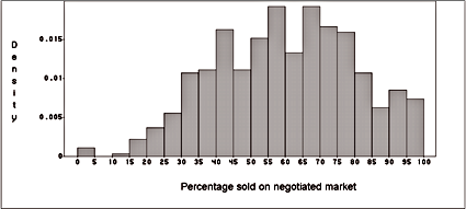
- 2.3
-
The two sub-markets (auctions and negotiated) have an equal
importance: a first analysis reveals that the same people are
transacting on these two "sub-markets" and that the same types of
fish are sold through both mechanisms. The trades concern 80
species of fish. Between 37% and 54% of each of the four main
fish species are sold on the auction market which suggests an
equivalent distribution of the production between the two market
mechanisms. The figure 1 clearly shows
that significant percentages of the production are traded on both
markets each day. 19000 tons are sold through auctions while
24000 tons are exchanged through the negotiated market. Around
60% of the transactions are made per year, on the negotiated
market and this proportion is stable through the period considered.
This proportion stays more or less the same when one considers the
quantities 63% or the value 66%. If the aggregate behavior
exhibits a stable repartition over days through the two sub markets,
our study shows further that most of the individuals switch over time
from one market to the other.
- 2.4
-
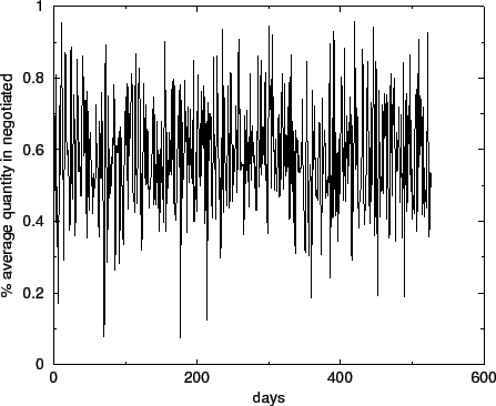
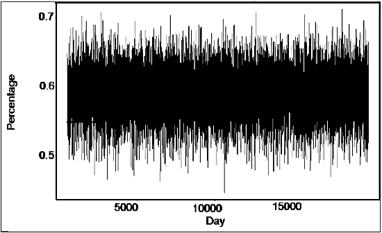
Figure 2 displays the percentage of the average quantity
played on the negotiated market.
Figure 3: The negotiated market: This graph exhibits the percentage of the quantity sold on the negotiated market each week. 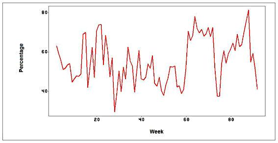
- 2.5
-
The Augmented Dickey-Fuller test for unit root rejects the null
hypothesis, meaning that the process is also stable. The lagged level of the
series t - 1, thus, provides some relevant information in predicting
the change in t.
- 2.6
-
Moreover, to analyze the co-movement between the
daily quantities sold in the negotiated and those sold in the
auction, we have studied the correlation between these quantities. A
significant positive correlation (+0.52) demonstrates the
co-movement and the stability of this aggregate relation.
In other words, when the whole quantity increases, the quantities played
on each market increase in absolute value.
Instead, looking at the
individual level we find very different behaviors.
- 2.7
-
In Figure (3) we look at the percentage of the quantity sold on negotiated market each week,
in order to remove weekly effects, and reduce the influence of 'extreme' days where very small quantities are sold.
The switching
-
- 3.1
-
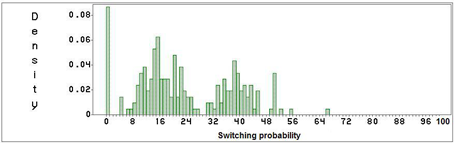
Figure 4 represents the distribution of the probability to switch from a market system
to the other, that is to say the probability for a seller to put the majority of his product on one market one day,
and on the other market the next time they come.
We can observe three peaks in the distribution, each representing one sellers' group. The ones that never switch are the sellers that only came a very small number of times on the market, and consequently did not have the opportunity to switch. Then we have two groups: the more 'switching' one is composed of the boats selling mainly on auctions, and the more stable one of the sellers going mainly on the negotiated market.
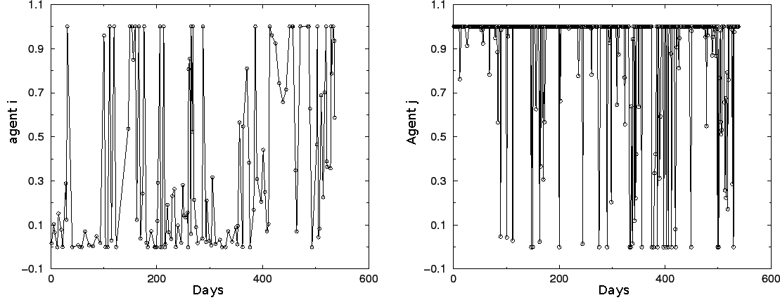
Figure 5 shows the percentage of the quantity sold on the negotiated market by two generic fishermen1. What is clear is the heterogeneity of the individual strategies. While the fisherman j (right side) plays mainly on the negotiated market, the agent i (left side) is more switching between the two sub-markets. - 3.2
-
Choosing the sales mechanism (auction or negotiated)
seems to be a strategic tool for sellers. Figure
6 reveals that among the biggest sellers,
two main strategies dominate, one which consists to sell mostly on
the negotiated market, another one which consists to sell less
than 45% on this market.
Figure 6: The negotiated market: distribution of quantities purchased by the 100 biggest sellers on each market. Two main strategies dominate, selling mostly on the negotiated market, or selling less than 45% on this market. 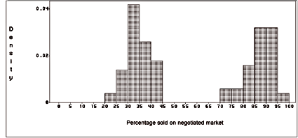
- 3.3
-
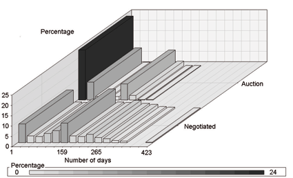
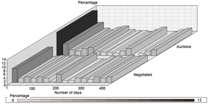
When we look at the presence of both sellers and buyers on the
two sub markets (cf. Figure 7), what can be observed
is that there are more people playing rarely on the auction market
than on the negotiated one (especially on the sellers side). This
could indicate a need to come often on the negotiated market to be
efficient on it, a need that doesn't exist on the other market. This
evidence seems in line with what some papers in financial literature
claim,
the auction organization being more efficient for less informed agents (cf. Viswanathan & Wang 2002)
- 3.4
-
We have now observed that the sellers adopt different strategies,
some mainly selling on the auction market, some mainly selling on the
negotiated market and most of them switching from one market to the
other. Two important questions are, first to understand what
determines the choice of the main market, then to explain the
switching process.
Characteristics of prices distributions
- 4.1
-
This section explores the particularities of the two prices
distributions (the one on the auction market, the other one on the
negotiated market) in the aim to better understand what drives the
fishermen strategies.
- 4.2
-
The price index used in this paper corresponds to a classic Paasche index.
For each day t it is calculated :
pi being the unit price of one transaction, qi the quantity sold in this transaction, and N the number of transaction made on this day.
- 4.3
-
The prices distributions are analyzed on the two markets,
separately for each group of sellers. The ones selling mainly on
auctions and the ones mainly on negotiated as seen on
figure (6). The analysis is driven for all
the transactions daily prices, which means that the goods are
heterogeneous. Figures (8) and
(9) show the distribution
for the two markets and for each group.
Figure 8: Price distributions on auction (left) and negotiated (right) markets for sellers going mainly on auctions 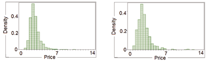
Table 1: Daily prices descriptive statistics for sellers going mainly on auctions
Auction Market Negotiated Market kurtosis 9.7 11.9 skewness 2.33 2.67 Median 2.43 2.46 St.Dev 1.06 1.39
- 4.4
-
When it comes to sellers that put the majority of their
products on the auction market it can be observed
(table 1) that the median price is slightly higher for
them on the negotiated market, but with a higher standard deviation and skewness indicating higher volatility and rarer large gain events,
making the decision to go to this market riskier. It is then clear
that at least for risk-adverse agents, going on the auction market can be a better strategy.
Figure 9: Price distributions on auction (left) and negotiated (right) markets for sellers going mainly on negotiated 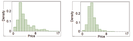
Table 2: Daily prices descriptive statistics for sellers going mainly on negotiated
Auction Market Negotiated Market kurtosis 2.02 4.0 skewness 1.45 1.39 Median 3.23 3.32 St.Dev 2.76 1.46
- 4.5
-
Otherwise, for sellers going mainly on negotiated, it can be observed in table 2 that the median price is slightly higher on the negotiated market, when the skewness and the standard deviation are higher on the auction market. Less risky and insuring slightly higher expected prices, the negotiated market is here more interesting.
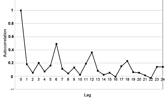
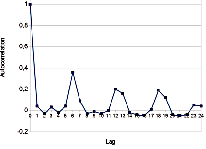
Figure 10 plots an autocorrelation on the prices of the negotiated market for all transactions, it shows one important fact: prices have a weekly trend (The market is opened six days a week), meaning there is a strong correlation between two successive Mondays (the same for the other days of the week). This tendency is weaker for the auction market (Figure 11) than for the negotiated one, confirming the hypothesis that going on this market is more strategic.
 ))
))
The prices/ quantities relation
- 5.1
-
The properties of the prices/quantities relation are now explored.
The relationship between price and quantity is the usual negative one,
but econometric evidence also reveals that quantities do not explain all the prices.
- 5.2
-
Looking a bit further into sellers behavior, a negative correlation appears between the
quantities sold on one market one day and the prices obtained on the
other market the day before.
- 5.3
-
Figure (12) shows the existence of a negative
relation at the aggregate level between the average price and total
quantity.
The relation of the figure (12) is well fitted by a logarithmic function with intercept 10.26, correlation coefficient -0.48 and slope -0.67 as seen in Figure(12) (red line). A simple logarithmic regression allows us to confirm the robustness of the negative price-quantity relation. The result is shown in the table 3.
Figure 12: Price-quantity relationship on the negotiated market. We plot average daily price and total daily quantity (black line) and the logarithmic function best fit (red line). 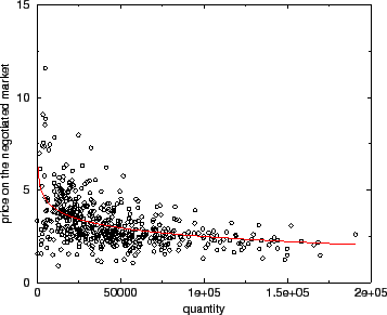
- 5.4
-
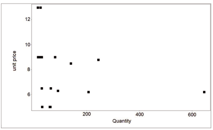
However, this aggregate behavior does not always have a
counterpart in the microeconomic data. Indeed plotting the data for
some single agent often yields a rather different picture with no
exact negative price quantities correlation. We show this phenomenon
in figure (13) (left side). In other situations,
although we observe a reduction in the price volatility for
increasing quantities, the price has not a clear trend, as shown in
figure (13) (right side).
As we saw earlier, (6), each seller selling mainly
in one sub-market, the scale of the quantities is of course completely different for the two
figures.
Figure 13: Price-quantity relationship for agent 87 on auction and negotiated market for the sole specie. 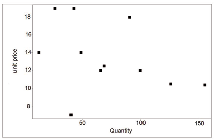
- 5.5
-
We now explore the cross relation
between prices on one market, one week and quantities on the other
market the other week.
(
 -
-  )
)  (| PStA - PStN| - | PSt+1A - PSt+1N|)
A designs the auction market, N the negotiated one. St and St+1 two successive weeks.
- 5.6
-
A significant negative correlation is found
between these two measures. When the global quantity increases, the
prices difference between the two markets decrease.
- 5.7
-
The empirical study has now suggests that, concerning the sellers,
going on one market or the other clearly results from a strategic
choice. For some of them, going on the auction market is more
interesting than going on the negotiated one, while the inverse is true
for some others. We also point out that, despite this evidence,
most of the fishermen switch from one market to the other. The
following section proposes an artificial agent based model to show
how this switching, which can seem erratic at a micro point
of view, allows a stable macro behaviour.
The artificial fish market
- 6.1
-
An artificial model 2 seeks to
reproduce possible strategies of agents on the studied market,
focusing on the switching process underlined in section 2.
It is shown in section 4 that even if sellers can be
divided in two groups,
each having a
distinct favorite market, they all switch from one market to the other more or less
frequently.
In what follows, we will not try to explain why one agent prefers one
market, but why all agents switch from one to the other.
- 6.2
-
The main goal here is to understand how the interactions
of different agents, heterogeneous in their strategies, are
able to generate the stable global behavior shown in the real data.
- 6.3
-
The statistical analysis has shown that, in absolute value, when the whole
quantity increases, the quantities played on each market also increases.
In relative value, we consider that the switching implies to modify the proportions.
Based on the assumption that the auction market plays a benchmark role
(fixing the competitive price), a
simplifying rule consists here in
exclusively analyzing what happens on the negotiated market.
- 6.4
-
To support this assumption, we have shown with figure
11 and figure
10 that the autocorrelation on this
sub-market is stronger, meaning that the decision will be taken using
mainly data acquired on the negotiated market, as it is more
meaningful, than information acquired on the auction market. We don't
try to reproduce the weekly trend, which is of no importance in the
mechanism studied in this paper.
Heterogeneous levels of information
among people are considered, through two main types of behaviors,
i.e. noisy agents and myopic ones. Myopic agents regularly revise
their strategies, following simple learning rules, as explained
below. Noisy agents are zero-intelligent agents: the introduction of
these agents is a simplification to describe different agents'
strategies that we do not investigate. In particular, agents can use
very dissimilar approaches and the zero-intelligent assumption
mirrors these heterogeneous human behaviors, not explicitly modeled
here. In this way we are close to the tradition of noisy strategies
as in Becker (1962) and Gode & Sunder (1997).
- 6.5
-
Prices are negotiated through buyers and sellers, following the
simple rule of "take it or leave it price". They are not posted and
agents are or sellers or buyers. The market is characterized by a continuous
decentralized search, generating out-of-equilibrium dynamics. Due to
the absence of any exogenously imposed market-clearing mechanism, the
economy is allowed to self-organize towards a spontaneous order with
persistent involuntary unsold fish and excess individual demands.
- 6.6
-
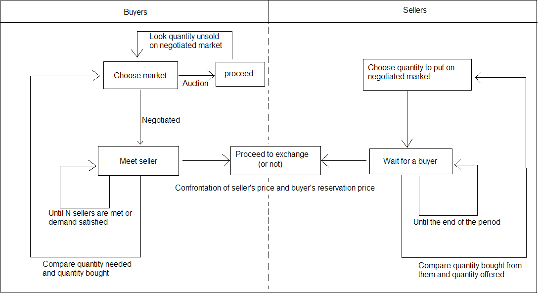
The overall functioning of the artificial market is shown in 14.
Equations used in the simulation follows.
- 6.7
-
The sellers, given their total quantity of fish, decide the
percentage to sell on the negotiated market.
Agents' choices are
simultaneous.
The time: Time is discrete, denoted by t = 0, 1, 2,.., T.
The buyers: j = 1,.., n buyers arrive at each period with a random divisible demand Dj. They meet a finite number k of sellers at random. If the price asked by the seller is lower than the reservation price 3 of the buyer, the transaction occurs. If the buyer's whole demand is not satisfied after he has visited k sellers, he is rationed. Each buyer j determines his reservation price rnegj according to
with xj a constant individual variable. With this function, most people have a low reservation price, while some of them have a high one. is a parameter of the model without real importance. It just
indicates the market price scale.
is a parameter of the model without real importance. It just
indicates the market price scale.
The sellers: At time t, i = 1,.., m sellers arrive on the market with a random constant supply Si that he divides between the auction market ( Sauct, i) and the negotiated one ( Snegt, i). - 6.8
-
To determine those quantities a seller uses the demand observed on the previous time step
as shown in equation 7.
- 6.9
-
Each seller i determines his price
pnegt, i as a function of the
daily global quantity offered on the negotiated market.
- 6.10
-
At the end of each period, a myopic seller revises his price according to the difference between the
expected demand and the observed one (equation 5). The parameter
 is then modified (equation 6).
(
 is a parameter for the learning. The higher it is the stronger the corrections will be made at each timestep)
The decision process: A myopic seller increases his supply Snegt, i if the demand at the previous time step was bigger than his previous supply, the quantity offered on the negotiated market is then defined in equation 7
The probability for a buyer to leave the negotiated
market is equal to
for a buyer to leave the negotiated
market is equal to
This means that the higher his excess demand at the end of the time step, the higher the probability he switches for the next period. ( Sneg, jt, i being the quantity exchanged on negotiated market between buyer j and seller i) - 6.11
-
A buyer has a probability
 to switch back to the negotiated market which depends on the level of
competition there. The higher is the excess demand on the negotiated
market at the end of time t,
the more likely a buyer is to come back a time t + 1.
to switch back to the negotiated market which depends on the level of
competition there. The higher is the excess demand on the negotiated
market at the end of time t,
the more likely a buyer is to come back a time t + 1.
- 6.12
-
Noisy agents play at random.
 )) with 0.5 < xj < 1
 )) with 0 <
 ))
))
The simulation results
- 7.1
-
The simulation parameters seek to fit the real conditions.
(Changing them would modify such things as the price scale or the average percentage of the quantity
on each market but not the overall dynamic)
200 sellers and 100 buyers are generated.
13% of sellers and 10% of buyers adopt random or noisy strategies,
which corresponds to the percentage of agents
(respectively buyers and sellers) coming very irregularly
on the real market (as shown in 2).
The individual supplies
are uniformly distributed in the interval
Si
 [0, 60] and
the individual demands are uniformly distributed in the interval
Dj [0, 120]. The number of sellers each buyer can link with
is k = 20.
is equal to 0.1, to 3 and
[0, 60] and
the individual demands are uniformly distributed in the interval
Dj [0, 120]. The number of sellers each buyer can link with
is k = 20.
is equal to 0.1, to 3 and  to 5.
to 5.
The results reported here are the outcome of simulations of T = 20000 periods. In order to get rid of transients, the first 500 simulated periods have not been considered.
- 7.2
-
Consistent with the empirical analysis, the
figure (15) shows, on the simulated scenario,
the existence of the negative relation (red line on the figure) at
the aggregate level between prices and quantities, even if this
relation is not clear at a micro level.
Figure 15: Price-quantity relationship on the simulated market (black dots) and the linear regression best fit (red line): the slope value is at -0, 62. 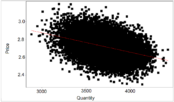
- 7.3
-
The simulated model reproduces the same stable aggregate behavior of
switching between the two sub-markets as in the real market.
Figure. (16) displays the percentage of the average quantity
played on the simulated market. We obtain a mean of 0.575% sold on
the negotiated market with a standard deviation of 0.046. (Compared
to a mean of 0.58% and a standard deviation on 0.154 for the
real market)
- 7.4
-
The stability of the process is
confirmed by the Augmented Dickey-Fuller test for unit root which
rejects the null hypothesis.
Figure 17: Percentage of the average quantity on the simulated negotiated market for 100 periods taken at random. 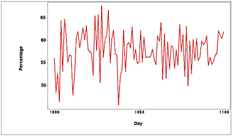
- 7.5
-
Figure (17) can be compared with figure
(3). We observe a higher
volatility on the real market: this can easily be explained by the
heterogeneity both of goods and overall quantity sold
that doesn't exist in the simulation.
- 7.6
-
Given the heterogeneity of individual strategies, we can confirm that this aggregate relation
derives from the interaction of multiple strategies. Unsold
quantities remain at a quite high level in our model (around 18%),
much higher than in reality, but this is easy to explain because of
the simplicity of the learning process. In the real market, people
revise their reservation prices all along a market day, which is not
the case in the simulated market. Our result could be easily
improved, allowing agents to continuously revise their price.
Conclusion
- 8.1
- The question of efficiency of market organization is an important one in economics. When theoretical results suggest the dominance of auctions, empirical studies present more mitigated results putting forward that the global efficiency depends on agents' characteristics and market environment. This article brings to light some important features concerning the role of market designs and the behaviour of agents facing these different mechanisms. The Boulogne s/mer fish market is a great field of experiment for better evaluating the role of market mechanisms in the allocation of resources. Our empirical study points out that for a fisherman, going on one sub-market or on the other is a strategic decision. It seems that this decision depends on the intrinsic characteristics of the agents, on the type of fish they mainly sell and on the global market environment. For some of them, it is usually more advantageous to sell on the auction sub-market, for some others the negotiated segment is more interesting. Despite of this, most of them frequently switch from one place to the other. The days where the whole quantity to sell is high, people prefer to go to the auction market, even if they are more often on the negotiated one. Reversely, when the fish is scarce, the agents go to the negotiated market, even if they are more of the "auction type". This is new, compared to the main results in the economic literature (which evaluates the mechanisms performance conditional to the economic environment, but does not envisage these switching opportunities). Focusing on the understanding of the switching process more than on the performance of the different market mechanisms, we propose an agent-based model which establishes conditions under which this switching is globally rational, leading to a constant and stable aggregate behaviour when the decision variable is the price. The rules adopted in the agent-based representation are directly derived from the empirical observation. As shown in the empirical part, in the real market, the whole quantity influences the individual decisions in terms of prices and shares of quantity. This observation is crucial and supports the modelling of the switching process in the artificial market.
- 8.2
- Modelling two types of individuals, some behaving under imperfect information but endowed with simple learning rules and some zero-intelligent others, we show that switching, which seems erratic at a micro level, can be a stable efficient strategy, when the coherence of the market is considered. What is interesting here, is to observe through the empirical analysis, that even if this relation is not always true at a micro level, it is consistent at the macro level, and this is in keeping with Hildenbrand's postulate. The simulation clearly reproduces the macro tendency, without any need for particular constraints at the micro level. The dynamic of the system seems then to generate a spontaneous organized structure, without any need of coordination. Thus, the macroscopic outcomes of this market are not directly derived from any of the individual components involved, but are the self-organized outcomes of the agents interaction. The simple interaction of noisy and myopic agents leads the system to stabilize itself despite of the market organization. It is not easy here to say which type of design (auction or negotiated) dominates the other. But it seems that the agents continuously adapt themselves and use the best mechanism conditional to the temporarily global environment of the market: and this explains the switching.
Acknowledgements
- We wish to thank Mauro Gallegati, Giulio Bottazzi and Mirta Gordon for helpful comments and suggestions. We acknowledge the editor and two anonymous reviewers for their helpful comments. Errors remain ours.
Notes
- 1
- We show the percentage of the average quantity for sellers 644073 (left side) and 87 (right side). However we have investigated this behaviour for 20 agents selected randomly, finding heterogeneous characteristics.
- 2
- This artificial market is coded in C++ language, and not using any specific tool or software.
- 3
- The price above which the buyer will not accept to trade.
References
-
ARTHUR, B. W. (1989)
'Competing
technologies, increasing returns, and lock-in by historical events.', Economic Journal 99(394), 116-131. [doi:10.2307/2234208]
BECKER,, G. S. (1962) 'Irrational behaviour and economic theory', Journal of Political Economy LXX, 1-13. [doi:10.1086/258584]
BOTTAZZI, G., Dosi, G. & Rebesco, I. (2005) 'Institutional architectures and behavioral ecologies in the dynamics of financial markets', Journal of Mathematical Economics Special Issue on Evolutionary Finance 41(1-2), 197-228. [doi:10.1016/j.jmateco.2004.02.006]
BULOW, J. & Klemperer, P. (1996) 'Auctions versus negotiations', The American Economic Review 86, 180-194.
Chena, S.-H., Lux, T. & Marchesi, M. (2001) 'Testing for non-linear structure in an artificial financial market', Journal of Economic Behavior & Organization 46(3), 327-342. [doi:10.1016/S0167-2681(01)00181-0]
CHIARELLA, C. & Iori, G. (2002) 'A simulation analysis of the microstructure of double auction markets.', Quantitative Finance 2(5), 346-353. [doi:10.1088/1469-7688/2/5/303]
GALLEGATI, M., Giulioni, G., Kirman, A. & Palestrini, A. (2011) 'What's that got to do with the price of fish? Buyer's behavior on the Ancona fish market.', Journal of Economic Behavior and Organization 80, 20-33. [doi:10.1016/j.jebo.2011.01.011]
GODE, D. K. & Sunder, S. (1993) 'Allocative efficiency of markets with zero-intelligence traders: Market as a partial substitute for individual rationality', The Journal of Political Economy 101, 119-137. [doi:10.1086/261868]
GODE, D. K. & Sunder, S. (1997) 'What makes markets allocationally efficient?', The Quarterly Journal of Economics 112(2), 603-630. [doi:10.1162/003355397555307]
GRANDMONT, J.-M. (1987) 'Distributions of preferences and the "law of demand"', Econometrica 55, 155-161. [doi:10.2307/1911161]
HILDENBRAND, W. (1994) Market Demand, Princeton: Princeton University Press. [doi:10.1515/9781400863716]
HOFFMANN, A., Jager, W. & Eije, J. V. (2007) 'Social simulation of stock markets: Taking it to the next level', Journal of Artificial Societies and Social Simulation 10(2)7 https://www.jasss.org/10/2/7.html.
KIRMAN, A. (2010) Complex Economics: Individual and Collective Rationality, Graz Schumpeter Lectures.
KIRMAN, A., Moulet, S. & Schulz, R. (2008) 'Price discrimination and customer behaviour: empirical evidence from Marseille', GREQAM document de travail 57.
KIRMAN, A. P. (1995) 'Economies with interacting agents', Discussion Paper Serie A 500, University of Bonn, Germany.
KIRMAN, A. & Vignes, A. (1990) Price Dispersion: Theoretical Coordination and Empirical Evidence from the Marseilles Fish Market, Macmillan.
MILGROM, P. (1986) Advances in Economic theory : Fifth world congress of the Econometric Society, Cambridge University Press, London: Macmillan, 11 - 32.
MILGROM, P. (2004) Putting auction theory to work. Cambridge University Press. [doi:10.1017/CBO9780511813825]
POGREBNA, G. (2006) 'Auctions, versus bilateral bargaining : Evidence from a natural experiment', Working Paper, available at SSRN http://ssrn.com/abstract=954891 .
SALLANS, B., Pfister, A., Karatzoglou, A. & Dorffner, G. (2003) 'Simulation and validation of an integrated markets model', Journal of Artificial Societies and Social Simulation 6(4)2 https://www.jasss.org/6/4/2.html.
STIGLITZ, J. (2004) Comments, in Milgrom, P. Putting auction theory to work. Cambridge University Press.
TAKAHASHI, H. & Terano, T. (2003) 'Agent-based approach to investors' behavior and asset price fluctuation in financial markets', Journal of Artificial Societies and Social Simulation 6(3)3 https://www.jasss.org/6/3/3.html.
TEDESCHI, G., Gallegati, M., Mignot, S. & Vignes, A. (2011) 'Lost in transactions: The case of the Boulogne s/mer fish market', Physica A: Statistical Mechanics and its Applications 391(4), 1400-1407. [doi:10.1016/j.physa.2011.09.035]
TEDESCHI, G., Iori, G. & Gallegati, M. (2009) 'The role of communication and imitation in limit order markets', European Physical Journal B 71(4), 489-497. [doi:10.1140/epjb/e2009-00337-6]
VIGNES, A. & Etienne, J.-M. (2011) , 'Can an exchange market be studied as a seller-seller network? the case of the Marseille fish market', Journal of Economic Behaviour and Organization 80, 50-67. [doi:10.1016/j.jebo.2011.07.003]
VISWANATHAN, S. & Wang, J. (2002) 'Market architecture: limit-order books versus dealership markets,', Journal of Financial Markets 5(2) , 127-167. [doi:10.1016/S1386-4181(01)00025-8]
WEISBUCH, G., Kirman, A. & Herreiner, D. (2000) 'Market organization and trading relationships', The Economic Journal 110(463), 411-436. [doi:10.1111/1468-0297.00531]