Abstract

The beer production-distribution game, in short "The Beer Game", is a multiplayer board game, where each individual player acts as an independent agent. The game is widely used in management education aiming to give an experience to the participants about the potential dynamic problems that can be encountered in supply chain management, such as oscillations and amplification of oscillations as one moves from downstream towards upstream echelons. The game is also used in numerous scientific studies. In this paper, we construct a mathematical model that is an exact one-to-one replica of the original board version of The Beer Game. We apply model replication principles and discuss the difficulties we faced in the process of constructing the mathematical model. Accordingly, the model is presented in full precision including necessary assumptions, explanations, and units for all parameters and variables. In addition, the adjustable parameters are stated, the equations governing the artificial agents' decision making processes are mentioned, and an R code of the model is provided. We also shortly discuss how the R code can be used in experimentation and how it can also be used to create a single-player or multi-player beer game on a computer. Our code can produce the exact same benchmark cost values reported by Sterman (1989) verifying that it is correctly implemented. The mathematical model and the R code presented in this paper aims to facilitate potential future studies based on The Beer Game.

Keywords:

Acquisition Lag, Artificial Agents, Beer Game, Mathematical Model, Replication, System Dynamics

Introduction

1.1

The beer production-distribution game, in short "The Beer Game", is a multiplayer board game, where each individual player acts as an independent agent. It was first introduced by Jay Forrester's System Dynamics (SD) research group of the Sloan School of Management at the Massachusetts Institute of Technology in the 1960s. The Beer Game is an application of SD modeling and simulation methodology, which is widely used in management education and aims to give an experience to the participants about the potential dynamic problems that can be encountered in supply chain management, such as oscillations and amplification of oscillations as one moves from downstream towards upstream echelons (Akkermans & Vos 2003; Barlas 2002; Chen & Samroengraja 2000; Forrester 1961, 1971; Größler et al. 2008; Sterman 2000). A detailed description of the original beer game, which is widely played by numerous people with different educational backgrounds and is also used in scientific studies, is given in Sterman (1989) and Croson and Donohue (2006). We list some of the work on The Beer Game to give an idea about the range of studies based on the game. Jacobs (2000) introduced the internet-based version of The Beer Game and reported that this version of the game significantly reduced the time required to play the game. According to him, the main reason for this difference is that in the board version of the game, participants manually keep the records of inventories and backlogs and calculate the total cost, but in the internet-based version of the game, the game software takes care of these calculations and does so in a faster and more accurate manner compared to human agents participating in the game. Day and Kumar (2010) used mobile phones to run the game and reported improved accuracy and speed due to the automated calculations. Independent from Jacobs' work (2000), Samur et al. (2004, 2005) developed a multi-player computerized version of The Beer Game. They first present verification runs to demonstrate that their model correctly represents the board game. Then they conclude that participants who played the board game were more successful than those who played the computerized version of the game. The potential causes for this result included the slower pace of progress of the board version, which gives more time to think about the order quantity, and the relatively more realistic environment of the board version. Steckel et al. (2004) examined the effect of reduced cycle times and the effect of shared point-of-sale (POS) information among the supply chain members in The Beer Game. They reported that reduced cycle times lead to reduced costs, which is an expected result. They further reported an interesting result that the benefit of POS information sharing depends on the customer demand pattern. Chaharsooghi et al. (2008) proposed a reinforcement learning (RL) model for ordering policies in supply chains and used The Beer Game model as an experimental platform. Kim (2009) extended The Beer Game into a supply network and conducted agent-based simulations in his study. Mosekilde and Laugesen (2007) conducted an extensive bifurcation analysis and showed that The Beer Game can produce complex dynamics. Thomsen et al. (1991) also showed that it is possible to obtain complex dynamics from The Beer Game, including hyperchaos.

1.2

The Beer Game is a four echelon supply chain consisting of a retailer, wholesaler, distributor, and factory, where each one of these echelons is managed by an independent agent. In this multi-agent game, there is an inventory control problem for each one of these echelons. During the game, every human agent in a team of four is responsible for one of the four echelons and manages the associated inventory by placing orders. The orders flow from downstream echelons towards upstream echelons and cases of beer flow in the opposite direction. The aim of the game is to minimize the accumulated total cost obtained by the participants of a team managing each echelon. The accumulated cost generated by each individual echelon is calculated at the end of the game by adding up all inventory holding and backlog costs obtained at the end of each simulated week (Sterman 1989).

1.3

At the beginning of an ongoing research study, a mathematical model that is an exact one-to-one replica of the original board version of The Beer Game, was needed. Moreover, we decided to use a model that had equations organized and executed in exactly the same order as the 'five steps' of the board game. We believed that such a model would facilitate the verification of our results and also potentially contribute to the analysis and understanding of the board game. We were not able to find a computer model in the literature that provided such an exact replica of the board game. Therefore, we first constructed a mathematical model that is independent from programming languages based on the descriptions of The Beer Game provided in Sterman (1989). Later, we coded this model in R^[1]. The mathematical model is given in full detail in the section named "Mathematical model of the beer game".

1.4

Axelrod (1997, pp. 20–21) noted that: "Replication is one of the hallmarks of cumulative science. It is needed to confirm whether the claimed results of a given simulation are reliable in the sense that they can be reproduced by someone starting from scratch." There are many other researchers who also emphasize the importance of replication as a validation approach (see for example, Edmonds & Hales 2003, 2005; Miodownik et al. 2010; Wilensky & Rand 2007). Model replication requires a significant effort because complex dynamic models are highly sensitive to the implementation details (Merlone et al. 2008). In his paper entitled "Advancing the Art of Simulation in the Social Sciences", Axelrod (1997) reports problems that were encountered in replicating simulation models described in other published work. According to Axelrod, some of the replication problems are caused by ambiguities, gaps, and errors in the model descriptions. Despite all the details provided by Sterman (1989), a significant effort was required to obtain a one-to-one mathematical replica of the board version of the game, and we experienced difficulties similar to the ones experienced by Axelrod (1997): (1) Sterman provided equations for the general stock management task, which can form a basis in obtaining The Beer Game equations. However, the exact equations for The Beer Game are not present in Sterman's paper, except for the ordering equation. (2) There is an ambiguity in the tie-breaking rule used in rounding the values of the orders. Hence, we are forced to assume a tie-breaking rule in rounding the values. (3) Expectation formation is assumed to be performed informally by a human participant in his mind and, therefore, is not listed among the five steps of The Beer Game. However, in the mathematical model, the decision making process is also captured as a part of the model and, therefore, we have to determine its place among the steps of the game. (4) There is an error regarding the conceptualization of the delay durations. In the section named "A discussion on acquisition lags", we explain the misconceptualization of the duration of acquisition lags that are present in the game and the error that can potentially be caused by it. Note that North and Macal (2002) also reported difficulties that they faced in their Beer Game docking process.

1.5

Although The Beer Game is an application of SD methodology, a one-to-one SD model of the game cannot be directly obtained because the order of calculations followed in the game and the order of calculations followed in SD methodology will not match unless the order of calculations in the corresponding SD model is carefully altered by introducing additional variables to the model. This mismatch also contributes to the difficulty in obtaining a complete mathematical model of the game. North and Macal (2002) implemented The Beer Game using three different platforms and they reported subtle differences in the outputs of those three different implementations, which we think those differences could only be eliminated by substantial amount of additional effort.

1.6

In the section named "R code of the mathematical model as an experimental platform", we provide an R code^[1] (R Core Team 2013) of the mathematical model presented in this paper to ease the simulation replications of our model. In the same section, we also shortly discuss how the code can be used in experimentation and how it can be used to create a single-player or multi-player beer game on a computer.

1.7

In Sterman (1989), the anchor-and-adjust heuristic formulation that is suggested to be used in decision making and the anchor-and-adjust heuristic formulation that is used in modeling the participant behavior are slightly different. In the section named "Verification of the mathematical model", we explain the differences between the two formulations, provide a different set of equations for the anchor-and-adjust heuristic formulation that is used in modeling the participant behavior, execute the corresponding R code^[2] with the optimum benchmark parameter values given by Sterman, and obtain the exact same benchmark cost values also presented by him. This process verifies that our R code is correctly implemented and it also validates that our model is a correct and exact representation of the board version of The Beer Game.

Mathematical model of the beer game

2.1

To conduct this research, we first constructed a mathematical model of The Beer Game based on a figure of the board game (see Figure 1 in this paper), equations, the five steps of the game, and descriptions given in Sterman (1989).

Figure 1. The Board of The Beer Distribution Game (Figure 2 in Sterman 1989, p. 327)

Parameters and initial values of the mathematical model

2.2

sati = 1 [week] for i = R, W, D, F

(1)

mdti = 1 [week] for i = R, W, D

(2)

sti = 2 [week] for i = W, D, F

(3)

plt = 2 [week]

(4)

Where sat (1/α_S in Sterman 1989) stands for the stock adjustment time, mdt stands for the mailing delay time, st stands for the shipment time, and plt stands for the production lead time. R, W, D, and F stand, respectively, for the retailer, wholesaler, distributor, and factory echelons (Figure 1). Note that sat, wsl, θ, and I* are the decision parameters (equations 1, 5, 6, and 10). The different sets of values of these parameters represent the different instances of the anchor-and-adjust ordering policy and, together with the decision making variables (equations 8, 9, 11–14, 47–50, 54–57, and 63–68), they define how the artificial agents make decisions. Note that the different sets of values for these parameters will not make the mathematical model divert from being an exact one-to-one replica of the original board version of The Beer Game.

wsli = 1 [dimensionless] for i = R, W, D, F

(5)

θi = 0.2 [1/week] for i = R, W, D, F

(6)

wsl (β in Sterman 1989) stands for the weight of supply line and θ (also θ in Sterman 1989) stands for the smoothing factor used by each echelon in the game in forming expectations using the simple exponential smoothing forecasting method. Theoretically, θ can take a value between 0 and 1.

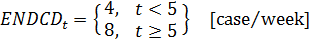
(7)

In the equation above, ENDCD stands for the end-customer demand. To save space, the unit case is used to represent a case of beer.

EECD0 = 4 [case/week]

(8)

EOi, 0 = 4 [case/week] for i = R, W, D

(9)

EECD stands for the expected end-customer demand, which is assumed to be calculated by the retailer. EO represents expected orders calculated by the wholesaler, distributor, and factory echelons based on the orders they receive from their respective customers (i.e., the retailer's orders received by the wholesaler, the wholesaler's orders received by the distributor, and the distributor's orders received by the factory).

Ii* = 0 [case] for i = R, W, D, F

(10)

(11)

(12)

(13)

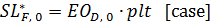
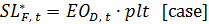
(14)

I* represents the desired inventory, and SL* stands for the desired supply line.

Bi, 0 = 0 [case] for i = R, W, D, F

(15)

Ii, 0 = 12 [case] for i = R, W, D, F

(16)

ITI1i, 0 = 4 [case] for i = R, W, D

(17)

WIPI10 = 4 [case]

(18)

ITI2i, 0 = 4 [case] for i = R, W, D

(19)

WIPI20 = 4 [case]

(20)

2.3

The equations 15 through 20 represent initial backlogs, initial inventories, and initial in-transit inventories (i.e., the values of the state variables at week zero). ITI2 (in-transit inventory 2) represents the shipping delay box just before the inventory box, and ITI1 (in-transit inventory 1) represents the shipping delay box before that (see Figure 1). The value of ITI1 belonging to an echelon is shifted to ITI2 of the same echelon after one simulated week. ITI2 is added to the inventory (I) or subtracted from the backlog (B) after a week. Likewise, WIPI1 and WIPI2 stand for work-in-process inventories. WIPI1 is the work-in-process inventory of the factory that will be shifted to WIPI2 after a week and that will eventually reach to the factory's inventory. WIPI2 is the work-in-process inventory that will be added to the factory's inventory (I_F) or subtracted from the backlog (B_F) after a week.

Oi, 1 = 4 [case/week] for i = R, W, D

(21)

PSR1 = 4 [case/week]

(22)

IOi, 1 = 4 [case/week] for i = W, D, F

(23)

O_i stands for orders that are placed by echelon i (retailer, wholesaler, and distributor). PSR stands for the production start rate, which is the production order given by the factory itself. IO_i stands for the incoming orders (the box right to the box of orders placed in Figure 1) that are received by echelon i. The purchase orders (O) placed by the retailer, wholesaler, and distributor and the production orders (PSR) given by factory at week t are placed for week (t + 1). Orders placed at week (t + 1) by the retailer, wholesaler, and distributor become the incoming orders (IO), respectively, for the wholesaler, distributor, and factory at week (t + 2). Therefore, the end-customer demand (ENDCD), which is given by Equation 7, orders (O), and production start rate (PSR) have no value at week zero, but they are assigned a value for the first time at week 1.

TCi, 0 = 0 [$] for i = R, W, D, F

(24)

uihc = 0.5 [$/(week·case)]

(25)

ubc = 1 [$/(week·case)]

(26)

TC, uihc, and ubc stand for the total cost generated by an echelon, the unit inventory holding cost, and the unit backlog cost, respectively.

2.4

The remaining model equations are given in an order based on the steps of the game presented in Sterman (1989). This sequence should strictly be followed while performing calculations to ensure an accurate representation of the board version of The Beer Game (Figure 1).

2.5

After initializing the board, the game facilitator declares the time as week 1, and the game starts from Step 1. After the completion of all steps (at the end of Step 5), the facilitator adds one week to the current time, declares it, and the game continues repeating the same process.

Step 1. Receive inventory and advance shipping delays

2.6

In The Beer Game, cases of beer flow from right to left (i.e., from the upper echelon to the lower) and orders flow from left to right (i.e., from lower echelon to the upper). In the first step of the game, the in-transit inventory (work-in-process inventory for the factory) that is immediately to the right of an inventory is added to the inventory by the participants. After that, the contents of the rightmost in-transit inventory boxes are shifted to the near-right in-transit inventory boxes, and the contents of the rightmost work-in-process inventory box are shifted to the near-right work-in-process inventory box. As a result, the rightmost in-transit inventory boxes and WIPI1 become empty.

Ii, t = Ii, t-1 + ITI2i, t-1 [case] for i = R, W, D

(27)

IF, t = IF, t-1 + WIPI2t-1 [case]

(28)

ITI2i, t = ITI1i, t-1 [case] for i = R, W, D

(29)

WIPI2t = WIPI1t-1 [case]

(30)

ITI1i, t = 0 [case] for i = R, W, D

(31)

WIPI1t = 0 [case]

(32)

2.7

Equations 31 and 32 are redundant in the sense that the exclusion of these equations will not prevent the correct simulation of the mathematical model, but we present them in order to follow the same exact process as in the board version of the game.

Step 2. Fill orders

2.8

In this step, each echelon calculates the amount of beer to be shipped to its customer (i.e., shipments from retailer to end customer, from wholesaler to retailer, from distributor to wholesaler, and from factory to distributor) by considering incoming orders from the customer, the backlog of orders, and the inventory of that echelon. After calculating shipments (S), each participant, except for the retailer, puts shipments to the boxes on their near left (i.e., ITI1_R, ITI1_W, ITI1_D, and WIPI1 are updated).

(33)

(34)

(35)

(36)

2.9

The shipment variables are flow variables in essence, and the unit of these variables is [case/week]. However, we use stock variables that have [case] as their unit in calculating the shipment variables. Therefore, corrections in the units are necessary. Accordingly, (1/week) and (1 week) are used in the shipment equations 33–36. These corrections have no effect on the numerical values, but they correct the units. To easily comprehend the issue, consider a car that traveled for one hour and covered 50 miles in this journey. In such a case, the average speed of the car during that one hour would be 50 miles per hour. Although the units of the distance covered by the car and its average speed are different, their numerical values are not. Note that, for similar reasons, we also use the same type of correction in many of the remaining equations. As a further explanation; in a discrete time model, the simulation time step becomes equal to the unit time of that simulation model. In such a model, when a numerical value with a unit of [items/time] accumulate for one unit time, the resulting numerical value will not change, but its unit will be [items].

ITI1i, t = Si, t · (1 week) [case] for i = R, W, D

(37)

WIPI1t = PSRt · (1 week) [case]

(38)

Step 3. Record inventory or backlog on the record sheet

2.10

After filling orders, participants either count their inventories if they have chips representing the cases of beer in their inventory boxes or calculate the backlogs if they fail to satisfy the totality of the past backlogs and the current orders received from their customers. They record the inventory or backlog on their record sheets. This is represented by the equations below:

BR, t = BR, t-1 + (ENDCDt − SENDC, t) · (1 week) [case]

(39)

BW, t = BW, t-1 + (IOW, t − SR, t) · (1 week) [case]

(40)

BD, t = BD, t-1 + (IOD, t − SW, t) · (1 week) [case]

(41)

BF, t = BF, t-1 + (IOF, t − SD, t) · (1 week) [case]

(42)

IR, t = IR, t − SENDC, t · (1 week) [case]

(43)

IW, t = IW, t − SR, t · (1 week) [case]

(44)

ID, t = ID, t − SW, t · (1 week) [case]

(45)

IF, t = IF, t − SD, t · (1 week) [case]

(46)

In this study, the equality sign is used in assigning values to parameters and variables, and it does not imply a mathematical equality. Therefore, the same variable can appear on left and right sides of the same equation (see, for example, equations 43–46).

Expectation formation

2.11

Expectation formation is assumed to be performed informally by a participant in his mind and, therefore, is not listed among the five steps of The Beer Game. Sterman (1989) modeled the expectation formation process using the simple exponential smoothing method (see Equation 9 in Sterman 1989). This process is reflected by the equations given below:

EECDt = EECDt-1 + θR · (ENDCDt − EECDt-1) · (1 week) [case/week]

(47)

EOR, t = EOR, t-1 + θW · (IOW, t − EOR, t-1) · (1 week) [case/week]

(48)

EOW, t = EOW, t-1 + θD · (IOD, t − EOW, t-1) · (1 week) [case/week]

(49)

EOD, t = EOD, t-1 + θF · (IOF, t − EOD, t-1) · (1 week) [case/week]

(50)

Step 4. Advance the order slips

2.12

Orders (O) placed by the retailer, wholesaler, and distributor become incoming orders (IO), respectively, for the wholesaler, distributor, and factory after a week.

IOW, t+1 = OR, t [case/week]

(51)

IOD, t+1 = OW, t [case/week]

(52)

IOF, t+1 = OD, t [case/week]

(53)

Step 5. Place orders

2.13

In the board version of The Beer Game, participants place orders and production requests in this last step. According to Sterman (1989), the decision making process of participants can be represented by using the anchor-and-adjust decision heuristic. The equations below (54–68) are all part of this heuristic, which finally results in orders and production requests. The retailer, wholesaler, and distributor place orders (equations 65–67) and the factory decides on the production requests (Equation 68). SL* stands for the desired supply line, EI stands for the effective inventory, SL stands for the supply line, SLA stands for the supply line adjustment, IA stands for the inventory adjustment, and PSR stands for the production start rate. The anchor of the anchor-and-adjust heuristic is the expected loss from the stock, which is EECD_t in Equation 65, EO_R,t in Equation 66, EO_W,t in Equation 67, and EO_D,t in Equation 68.

(54)

(55)

(56)

(57)

EIi, t = Ii, t − Bi, t [case] for i = R, W, D, F

(58)

SLR, t = IOW, t+1 · (1 week) + BW, t + ITI1R, t + ITI2R, t [case]

(59)

SLW, t = IOD, t+1 · (1 week) + BD, t + ITI1W, t + ITI2W, t [case]

(60)

SLD, t = IOF, t+1 · (1 week) + BF, t + ITI1D, t + ITI2D, t [case]

(61)

SLF, t = WIPI1t + WIPI2t [case]

(62)

(63)

IAi, t = (Ii* − EIi, t) / sati [case/week] for i = R, W, D, F

(64)

(65)

(66)

(67)

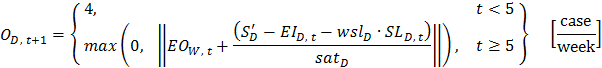
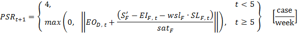
(68)

2.14

In the board version of the game, human agents give orders. However, in our model, artificial agents give orders as described by equations 65–68. All equations belonging to the five steps of the game (equations 27–69) are calculated for the current simulated week, except for the equations for incoming orders (51–53), orders (65–67), and production start rate (68). The equations for incoming orders, orders, and production start rate are calculated for the next simulated week. In the board version of the game, orders can only be integers. The rounding function (|| ||) used in equations 65–68 (and also equations 72–75) reflects this aspect of the game. In rounding the values, we assume that the "round half away from zero" tie-breaking rule is used.

2.15

In the original game, the accumulated total cost of each echelon is calculated at the end of the game from the record sheet kept by the participant managing that echelon. In the mathematical model, the total cost is calculated at the end of each simulated week using the equation given below:

TCi, t = TCi, t-1 + (uihc · Ii, t + ubc · Bi, t) · (1 week) [$] for i = R, W, D, F

(69)

2.16

After this final step, the simulated time is increased by one week and announced to the participants. The game continues by repeating the whole process starting from Step 1 until Step 5 of week 36 is completed. After the simulation ends, the main performance measure, which is team total cost (TTC), is calculated.

TTC = TCR, 36 + TCW, 36 + TCD, 36 + TCF, 36 [$]

(70)

R code of the mathematical model as an experimental platform

3.1

The R code^[1] (R Core Team 2013) of the mathematical model is ready to be executed; one needs to simply copy the code from the text file and paste it to R console in order to execute it. As mentioned before, equations 1, 5, 6, and 10 are the decision parameters (sat, wsl, θ, and I*) that describe the decision making processes of the artificial agents, and their different values represent different instances of the anchor-and-adjust ordering policy. Hence, one can change the values of these parameters in the code without making the mathematical model divert from being an exact one-to-one replica of the original board version of The Beer Game. After the change, one can re-execute the code to obtain the corresponding cost values. The weekly values of any variable can easily be displayed by simply typing the name of that variable in R console. In this way, the code serves as an experimental platform. One can also generate graphical outputs using the code^[3]. We set sat = 2, wsl = 0.8, θ = 0.4, and I* = 0 for all echelons to obtain the example dynamics presented in figures 2–4.

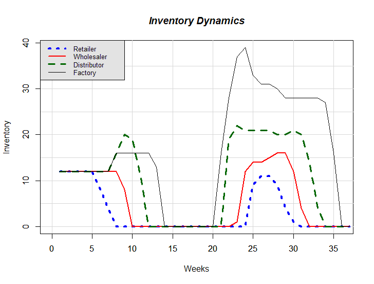
Figure 2. An example of Inventory Dynamics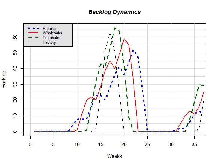

Figure 3. An example of Backlog Dynamics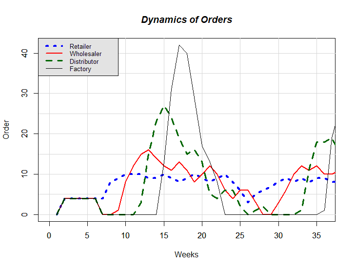

Figure 4. An example of Dynamics of Orders

3.2

To create different settings for a simulation experiment without altering the model structure, one can change the end customer demand pattern given by Equation 7 and play with the initial values of the stock variables, but those changes will imply a diversion from the original setting of The Beer Game. The model structure can also be altered. For example, one can change the delay times mdt (mailing delay time), st (shipment time), or plt (production lead time). However, such a change would imply an increase or decrease in the number of the associated variables. For instance, if one wants to increase the shipment time of an echelon from two weeks to three weeks, he must introduce one more in-transit inventory variable (i.e., ITI3). Another example could be the addition of production capacity to Equation 68 or the addition of shipment capacities to equations 33–36.

3.3

Simulation experiments can also be conducted in another programming environment by re-writing the code using that programming language. One can also develop a multi-player beer game using a programming environment that supports user interface creation. In that case, the respective order equations describing the artificial agents' decision making processes should be removed from the code and four human agents would be asked to insert values for orders of the four echelons. Alternatively, a single-player version of the game can be constructed. In this case, a human agent would give orders for one of the four echelons and three artificial agents would control the orders of the remaining echelons.

A discussion on acquisition lags

4.1

In The Beer Game, the acquisition lag is the summation of the mailing delay time and shipment time for the retailer, wholesaler, and distributor, and it is directly equal to the production lead time for the factory. In the game, orders placed by an echelon (i.e., the retailer, wholesaler, or distributor) at week t will reach the inventory of that echelon at week (t + 4) given that the supplier of that echelon has sufficient inventory to fulfill the order. For the factory, orders given at week t will be received at week (t + 3). Therefore, Sterman (1989) states many times in his paper that the acquisition lag for the retailer, wholesaler, and distributor is at least 4 weeks, and it is always 3 weeks for the factory. However, we claim that orders placed at Step 5 of week t are for week (t + 1) (see equations 21, 22, 65-68, and 72-75). Therefore, slightly changing the game, by placing orders at the beginning of Step 1 of week (t + 1) instead of placing them at the end of Step 5 of week t, will make no difference. Accordingly, in our mathematical model, the acquisition lags used in calculating the values of the desired supply line are 3, 3, 3, and 2 weeks for the retailer, wholesaler, distributor, and factory, respectively (see equations 2–4, 11–14, and 54–57). In the desired supply line equations (11–14 and 54–57), which correspond to Equation 7 in Sterman (1989), using acquisition lags of 4 weeks (for the retailer, wholesaler, and distributor) and 3 weeks (for the factory) instead of 3 weeks (for the retailer, wholesaler, and distributor) and 2 weeks (for the factory) will create a steady-state error in the dynamics.

Verification of the mathematical model

5.1

After constructing a one-to-one model of The Beer Game, we entered the optimal decision parameter values suggested by Sterman (1989) into our model. These parameter values are 0, 1, and 1 for θ (smoothing factor; also θ in Sterman 1989), sat (stock adjustment time; 1/α_S in Sterman 1989), and wsl (weight of supply line; β in Sterman 1989), respectively, for all echelons. The other decision parameter given by Sterman is S', which is defined as I* (desired inventory; S* in Sterman 1989) plus wsl times SL* (desired supply line; SL* in Sterman 1989); see Equation 71 and the unnumbered S' equation in Sterman (1989, p. 334). Sterman gives the optimal values of S' as 28, 28, 28, and 20 for the retailer, wholesaler, distributor, and factory echelons, respectively.

Si' = Ii* + wsli · SLi* [case] for i = R, W, D, F

(71)

5.2

In our mathematical model, the SL* values are dynamically updated as the expected orders from the customers change. Thus, S' should also be a variable. However, Sterman uses constant SL* and S' values. If the S' value is used instead of separate I* and SL* values and if it is a constant, the order equations 65–68 become as follows:

(72)

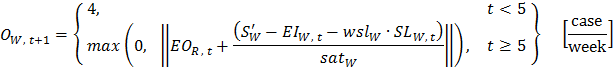
(73)

(74)

(75)

5.3

After simulating our model with the optimum θ, sat, wsl, and S' values using the order equations 72–75, we obtained the exact same benchmark cost values reported by Sterman, which supports our claim that our model is an exact representation of The Beer Game. Note that the conceptual error regarding the acquisition lags has no effect on the model used by Sterman in optimizing the parameters because S' is a constant; it is not dynamically calculated during the optimization runs. The R code of the mathematical model that is modified with and for the ordering equations 72–75 is also provided^[2]. In this version of the R code, sat, wsl, θ, and S' are the decision parameters (equations 1, 5, 6, and 71). The different sets of values of these parameters represent the different instances of the anchor-and-adjust ordering policy and, together with the decision making variables (equations 8, 9, 47–50, and 72–75), they define how the artificial agents make decisions.

5.4

As a final step in verification of the mathematical model, we first remove the ordering equations from the R code^{[1], [2]} and, instead, insert pseudo-random orders into the code. We also play the board version of the game with the same pseudo-random orders. The dynamics obtained from the R code and the board version of the game exactly match.

Conclusions

6.1

In this study, we constructed a detailed mathematical model that represents and replicates the exact execution order of the steps of the original board version of The Beer Game. As a part of the introduction section, we also state the difficulties that we faced in the construction process of such an exact one-to-one replica. One of the main difficulties is an error regarding the conceptualization of the delay durations as explained in detail in the section named "A discussion on acquisition lags". We present the constructed model in full precision including necessary assumptions, explanations, and units for all parameters and variables in the section named "Mathematical model of the beer game".

6.2

According to Axelrod (1997), internal validity (i.e., verification), usability, and extendibility are the three goals of the programming of a simulation model. To increase the usability of the model presented in this paper, we stated the adjustable parameters, mentioned the equations governing the artificial agents' decision making processes, and wrote an R code^[1] of the model. For extendibility, in the section named "R code of the mathematical model as an experimental platform", we shortly discussed how the code can be used in experimentation and how it can be used to create a single-player or multi-player beer game on a computer. For verification, we modified some of the equations belonging to the decision making formulations of the artificial agents and presented them in the section named "Verification of the mathematical model". We also modified the R code accordingly. Finally, we executed the modified R code^[2] with the optimum benchmark parameter values given by Sterman (1989) and obtained the exact same benchmark cost values also presented by him verifying that our R code is correctly implemented. This also validates that our model is a correct and exact representation of the board version of The Beer Game.

Acknowledgements

The authors thank Dr. Yaman Barlas, Dr. Nigel Gilbert, Dr. Gönenç Yücel, and the second referee of this article for their valuable suggestions.

This research is supported by a Marie Curie International Reintegration Grant within the 7th European Community Framework Programme (grant agreement number: PIRG07-GA-2010-268272) and also by Bogazici University Research Fund (grant no: 6924-13A03P1).

Notes

¹ The R code of the mathematical model can be found at http://www.openabm.org/model/4161/version/1/view

² The R code of the modified mathematical model can be found at http://www.openabm.org/model/4163/version/1/view

³ The R code of the mathematical model (code for graphical output added) can be found at http://www.openabm.org/model/4166/version/1/view

References

AKKERMANS, H. & Vos, B. (2003). Amplification in service supply chains: An exploratory case study from the telecom industry. Production and Operations Management, 12(2), 204–223. [doi:10.1111/j.1937-5956.2003.tb00501.x]

AXELROD, R. (1997). Advancing the art of simulation in the social sciences. Complexity, 3(2), 16–22. [doi:10.1002/(SICI)1099-0526(199711/12)3:2<16::AID-CPLX4>3.0.CO;2-K]

BARLAS, Y. (2002). System Dynamics: Systemic Feedback Modeling for Policy Analysis. In Knowledge for Sustainable Development: An Insight into the Encyclopedia of Life Support Systems (pp. 1131–1175). Paris, France and Oxford, UK: UNESCO/EOLSS.

CHAHARSOOGHI, S. K., Heydari, J. & Zegordi, S. H. (2008). A reinforcement learning model for supply chain ordering management: An application to the beer game. Decision Support Systems, 45(4), 949–959. [doi:10.1016/j.dss.2008.03.007]

CHEN, F. & Samroengraja, R. (2000). The stationary beer game. Production and Operations Management, 9(1), 19–30. [doi:10.1111/j.1937-5956.2000.tb00320.x]

CROSON, R. & Donohue, K. (2006). Behavioral causes of the bullwhip effect and the observed value of inventory information. Management Science, 52(3), 323–336. [doi:10.1287/mnsc.1050.0436]

DAY, J. M. & Kumar, M. (2010). Using SMS text messaging to create individualized and interactive experiences in large classes: A beer game example. Decision Sciences Journal of Innovative Education, 8(1), 129–136. [doi:10.1111/j.1540-4609.2009.00247.x]

EDMONDS, B. & Hales, D. (2003). Replication, Replication and Replication: Some Hard Lessons from Model Alignment. Journal of Artificial Societies and Social Simulation, 6(4), 11 <https://www.jasss.org/6/4/11.html>

EDMONDS, B. & Hales, D. (2005). Computational Simulation as Theoretical Experiment. The Journal of Mathematical Sociology, 29(3), 209–232. [doi:10.1080/00222500590921283]

FORRESTER, J. W. (1961). Industrial Dynamics. Waltham, MA: Pegasus Communications.

FORRESTER, J. W. (1971). Principles of Systems. Waltham, MA: Pegasus Communications.

GRÖßLER, A., Thun, J. H. & Milling, P. M. (2008). System dynamics as a structural theory in operations management. Production and Operations Management, 17(3), 373–384. [doi:10.3401/poms.1080.0023]

JACOBS, F. R. (2000). Playing the beer distribution game over the internet. Production and Operations Management, 9(1), 31–39. [doi:10.1111/j.1937-5956.2000.tb00321.x]

KIM, W.-S. (2009). Effects of a Trust Mechanism on Complex Adaptive Supply Networks: An Agent-Based Social Simulation Study. Journal of Artificial Societies and Social Simulation, 12(3), 4 <https://www.jasss.org/12/3/4.html>

MERLONE, U., Sonnessa, M. & Terna, P. (2008). Horizontal and Vertical Multiple Implementations in a Model of Industrial Districts. Journal of Artificial Societies and Social Simulation, 11(2), 5 <https://www.jasss.org/11/2/5.html>

MIODOWNIK, D., Cartrite, B. & Bhavnani, R. (2010). Between Replication and Docking: "Adaptive Agents, Political Institutions, and Civic Traditions" Revisited. Journal of Artificial Societies and Social Simulation, 13(3), 1 <https://www.jasss.org/13/3/1.html>.

MOSEKILDE, E. & Laugesen, J. L. (2007). Nonlinear dynamic phenomena in the beer model. System Dynamics Review, 23(2–3), 229–252. [doi:10.1002/sdr.378]

NORTH, M. & Macal, C. (2002). The Beer Dock: Three and a Half Implementations of the Beer Distribution Game. <http://backspaces.net/sun/SCSim/BeerDock.pdf>. Archived at: <http://www.webcitation.org/6LUrLLIVQ>.

R CORE TEAM. (2013). R: A language and environment for statistical computing. R Foundation for Statistical Computing. Vienna, Austria. <http://www.R-project.org/>

SAMUR, M. G., Eren, E. C., Hancer, O. & Tunakan, B. B. (2004). Testing Simultaneous Multiple Decision Maker Characteristics in a Dynamic Feedback Environment. B.Sc. Project, Bogazici University.

SAMUR, M. G., Eren, E. C., Hancer, O. & Tunakan, B. B. (2005). A computerized beer game and decision-making experiments. In Proceedings of the 23^rd International System Dynamics Conference. Boston, MA.

STECKEL, J. H., Gupta, S. & Banerji, A. (2004). Supply chain decision making: Will shorter cycle times and shared point-of-sale information necessarily help? Management Science, 50(4), 458–464. [doi:10.1287/mnsc.1030.0169]

STERMAN, J. D. (1989). Modeling managerial behavior: misperceptions of feedback in a dynamic decision making experiment. Management Science, 35(3), 321–339. [doi:10.1287/mnsc.35.3.321]

STERMAN, J. D. (2000). Business Dynamics: Systems Thinking and Modeling for a Complex World. Boston, MA: Irwin/McGraw-Hill.

THOMSEN, J. S, Mosekilde, E. & Sterman, J. D. (1991). Hyperchaotic phenomena in dynamic decision making. In E. Mosekilde and L. Mosekilde (Eds.), Complexity, Chaos, and Biological Evolution (pp. 397–420). New York: Plenum Press. [doi:10.1007/978-1-4684-7847-1_30]

WILENSKY, U. & Rand, W. (2007). Making Models Match: Replicating an Agent-Based Model. Journal of Artificial Societies and Social Simulation, 10(4), 2 <https://www.jasss.org/10/4/2.html>