Abstract

This paper describes the process and results of validating a simulation model of agriculture for a region in New Zealand. Validation is treated as a process, in which simulation models are made useful for specific purposes by making them conform to observed historical trends and relationships. In this case, the model was calibrated to reproduce the year-by-year conversion to dairying from 1993 to 2012 in Southland, New Zealand. This was achieved by holding constant some elements of the simulation model, based on economic theory or data, and by running simulations on a range of values for two key parameters. The paper describes the model and process, and demonstrates that empirical validation is possible if approached pragmatically with a view to the intended use of the model. Important elements are: using stylised facts to limit the parameter space ex ante, establishing the range of model outcomes and focusing on the most likely parameter space, focusing the search for parameter values where there is the greatest uncertainty, and using historical data to calibrate models.

Keywords:

Agriculture, Interdisciplinary Research, Multi-Agent Simulation, Validation, Agent-Based Model

Introduction

1.1

Charles Macal presented the keynote address to the 14th International Workshop on Multi-Agent Based Simulation on 7 May 2013. He noted that one of the first questions any person who is presenting a model or its results will be asked is, "Has your model been validated?" Macal suggested that without the ability to say "yes", the model is unlikely to be adopted or used in practice. This situation raises several questions: what does "validated" actually mean in practice, can it be achieved and if so, how?

1.2

Some economists claim that meaningful validation is impossible (Windrum et al. 2007):

Socio-economic systems, it is argued, are inherently open-ended, interdependent and subject to structural change. How can one then hope to effectively isolate a specific 'sphere of reality', specify all relations between phenomena within that sphere and the external environment, and build a model describing all important phenomena observed within the sphere (together with all essential influences of the external environment)?

This viewpoint suggests that, because there are uncertainties and complexities, model validation is impossible. An alternative viewpoint argues instead that validation for social science modelling is shades of grey rather than black or white. Models of human behaviour are not precluded from "validation", but the validation is an on-going process in building trust in the model and its ability to provide insights into the research questions at hand. Macal (2013) expressed this view succinctly:

The goal of model validation is to make the model useful in the sense that the model addresses the right problem, provides accurate information about the system being modelled, and … helps to [ensure] the model is actually used.

It is perhaps not surprising then that the literature suggests a wide range of validation approaches, but as Fagiolo et al. (2006, p. 9) stated, "There is no consensus at all about how (and if) AB [agent-based] models should be empirically validated." The intent and process of validation is thus a contested area of research.

1.3

This paper provides an example of model validation. The main validation exercise was to compare actual past land-use change to land-use change produced by the model, similar to Bell (2011). Land use and land-use change is a key driver of both rural economies and environment impacts of agriculture. For agricultural modelling generally and the present research in particular, modelling land use is a useful purpose as defined by Galan et al. (2009) and sets the scope for the validation. To set the stage for the validation exercise, this paper reviews the literature on validation to uncover themes within the processes and approaches that have been adopted. The paper then describes how a multi-agent simulation (MAS) developed for modelling the Southland region of New Zealand was empirically validated, and draws some lessons about validation from that exercise.

Literature review

2.1

Validation is not a single thing, a unified concept or an agreed process. Instead, there are several processes targeting similar concepts, all working towards demonstrating that a model is useful for describing observed phenomena. This review describes different types or modes of validation: scope of validation, verification, theoretical validation, empirical validation, statistical validation and participatory validation.

2.2

A key issue is the scope of validation. A common theme is that validation is inextricably linked to the model's purpose or research question. Galan et al. (2009) noted, "For us, validation is the process of assessing how useful a model is for a certain purpose". The key phrase here is "for a certain purpose". Their validation aimed to show that a model is useful for a particular scope of questions. Targeting the validation to the outputs that matter for the research question is emphasised by Berger et al. (2010) and Macal (2013). The validation plan for any model therefore needs to be designed with the model's purpose in mind. Thus, model validity is contingent: a model is not universally valid, but valid for specific uses in specific contexts. The question, "has your model been validated?", is incomplete unless it specifies the context. Importantly, there is concern over whether "validation" is even a useful term, as it appears to mean different things to different people (Augusiak et al. 2014).

2.3

A second theme in the literature is verification, which answers the question "is the simulation working as you want it to do?" Galan et al. (2009) suggested verification is the process of looking for errors, where errors appear when a model does not comply with the specifications imposed by its own developer. Some, such as Marks (2013), suggest verification is separate from validation, and that the two combine to produce assurance. Verification goes by other names such as program validity (Richiardi et al. 2006) and internal validity (Bharathy & Silverman 2010). These terms point to the same aim: to ensure the model is accurately representing what the authors want it to. Some ways of achieving verification are testing and debugging model code, re-implementing code in different programming languages or on different computers, applying the model to very well understood examples, and creating extractions of the model (Galan et al. 2009). These examples emphasise that verification is procedural. It is demonstrated by following a processes and having a successful or satisfactory outcome.

2.4

Theoretical validation is a third theme widely discussed within this literature. Theoretical validation seeks to ensure the correct application of relevant theories within the model. Richiardi et al. (2006) described theory validity as the validity of the theory relative to the simuland (the real-world system). Schreinemachers and Berger (2011) note that one part of validation, which they refer to as "validation by construct" (based on McCarl and Apland 1986), is ensuring that the relationships within the model are based on sound theory. Macal (2013) comments that one component of validation is validating theory, which he defines as ensuring the technical relationships within the model are appropriately grounded. In a social science application, the relevant theories may touch on technology adoption behaviours, social networks, objective functions, production and expenditure functions. In agriculture, physical science theories may also be included, such as theories about the relationship of soil types to pasture productivity and environmental impacts.

2.5

Probably the largest theme is empirical validation. Fagiolo et al. (2006) provided three widely cited approaches for empirical validation: indirect calibration, the Werker-Brenner approach and the history-friendly approach. The steps involved for each of these approaches are directly taken from Moss (2008). In the indirect calibration approach, researchers identify macro-level "stylised facts" such as firm-size distributions or employment-growth relations. They then inform model design by "empirical and experimental evidence about microeconomic behaviour and interactions." The stylised facts are then used to provide ex ante restriction on the parameter space for the microeconomic functions, possibly by using Monte Carlo techniques. Indirect calibration identifies model parameters based on several sources of information – macro-level regularities plus available microeconomic estimates. In the Werker-Brenner approach, researchers use existing empirical knowledge to calibrate initial conditions and the ranges of model parameters. They then obtain simulation outputs for each set of parameter values for the model. From these outputs, they discard all sets of parameter values except those "that are associated to the highest likelihood by the current known facts (i.e. empirical realisations)." The surviving parameter sets together with domain expertise from "historians" are used to further constrain the parameter space of the model. The Werker-Brenner approach is similar to indirect calibration in that it combines different ways of knowing – empirically determined relationships plus domain expertise – but inverts the process to focus on the empirical data first and the "expertise" or "stylised facts" second. The history-friendly approach starts by designing the agents and interaction mechanisms on the basis of detailed empirical studies, anecdotal evidence and historical studies. These data are then used to assist "the identification of initial conditions and parameters on key variables likely to generate the observed history." Researchers then compare the model outputs (the "simulated trace history") to the observed history of the domain being studied. The history-friendly approach thus uses both micro-level and macro-level data, moving from the former to the latter.

2.6

Although there may be theoretical appeal in differentiating the three approaches, they do not seem to have been explicitly used in much of the practical validation literature. Villamor et al. (2012), who adopted the indirect calibration method in validating a land-use change model, is an obvious exception. While the order of application changes between approaches, the consistent message is to use empirical evidence, anecdotal evidence, stylised facts, and actual historical outcomes to limit the set of values for unknown parameters. They are essentially structured programmes for working towards convergent validity. Macal (2013) did suggest that validation can make use of critical cases or historical examples that can be used as natural experiments, but does not explicitly link the use of such examples to any specific validation approach as described by Fagiolo et al. (2006).

2.7

Statistical validation is yet another type of validation. Klügl (2008) explained the statistical rigour required to ensure the model is not just calibrated but validated: "calibration and validation must use different data sets for ensuring that the model is not merely tuned to reproduce given data, but may also be valid for inputs that it was not given to before." Empirical validation in social sciences sometimes struggles with this level of validation because controlled experiments cannot be performed on the system, and sometimes only a single historical dataset exists (Macal 2013). The difficulties with statistical validation may, in fact, have contributed to convergent validity approaches of Fagiolo et al. (2006) and described above.

2.8

A final theme gaining traction is interactive or participatory validation. Interactive or participatory validation involves the use of experts and/or stakeholders to act in the place of agents. The expert or stakeholder outcome can then be compared to the standard model simulation. Berger et al. (2010), for example, document interactive validation sessions for their linear-programming based MAS model. Their use of stakeholders uncovered constraints that had not previously been considered in the modelling. Once the new constraints were incorporated into the model, the expected land-use projections achieved a high degree of fit with that suggested by the stakeholders. Millington et al. (2011) completed a similarly participatory approach where interviewees were asked to identify shortcomings of their model, so that the model could be revised to more closely match the stakeholders' understanding of land-use change processes. Macal (2013) used a participatory simulation in validation of a complex electricity transmission and pricing model that allowed experts to place themselves in the positions of agents. This type of validation is not dissimilar to the use of historians in the Werker-Brenner approach to empirical validation (Fagiolo et al. 2006).

Model description

3.1

Agriculture is a complex system in which several agents act at different, nested levels, having impacts on their own environment; it is thus an appropriate field for agent-based modelling (Kaye-Blake et al. 2010). A MAS approach was selected for the present research for three principal reasons:

• to model decision heuristics other than optimisation: many economic and agricultural models assume that farmers maximise profit or income (e.g., Schreinemachers & Berger 2011), but the use of maximisation as to describe decisions has been contested (Rabin 2002; Simon 1955)
• as a framework to include data from different disciplines: the project aimed to include economic, social and biophysical information in workshops with stakeholders, and in particular to demonstrate the interactions between natural and social science information at the farm level (Berger et al. 2007). It also aimed to use empirical data wherever possible; Bell (2011) suggested there is only a small body of work using empirical data in agent-based models for agriculture
• as an intuitive and understandable approach: the inputs and outputs needed to be easy to communicate, and a MAS approach allows simple inputs like decision heuristics for economic decisions and production budgets for biophysical data. The MAS specifically used a driving forces – agents – land-use change schema (Hersperger et al. 2010) for linking inputs to farmer to their farming choices.

3.2

Conceptually, the model used in this research, RF-MAS (Rural Futures Multi-Agent Simulation), can be described by layers as shown in Figure 1. The initial layer is a dataset of farms that describes their locations, sizes and productive capacity as indicated by their Land Use Capability classes. The second layer is a set of production budgets for all the land uses in a region. Each farm is linked to all the land uses technically feasible on the property. This forms a set of options for the farm. The third layer is the farmer-agents in the model. Their social, economic and demographic parameters are based on statistics for the region, and their modelled behaviours are based on historical data and research on farmer decision making. Farmer-agents are presented each period with the possibility of choosing a new land use for the farm, given the set of feasible options. Their decisions determine land use for each farm, which then lead to regional economic and environmental consequences.

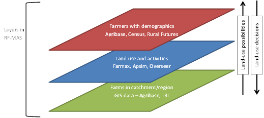
Figure 1. Conceptual design of RF-MAS

3.3

A model run follows a series of steps, which are described below and shown as flowcharts in Appendix A.

• Initialisation: farms and farmers are loaded into the model. Farms are read into the model from datasets based on Agribase (AsureQuality New Zealand, several years) and the Land Resource Inventory and Land Cover Database (2012). Farmers are generated from distributions of farmer demographics based on Agribase. Farms and farmers are assigned to each other on a one-for-one basis. Farmers are also assigned to peer networks built using the "Small World" algorithm (Jin et al. 2001), which is a mathematical representation of connectedness and clustering effects seen in social networks
• Pre-processing: farmers are aged by one year. Age affects several aspects of farmer behaviour. First, farmers above a certain age are likely to have children although not all do; this is assigned probabilistically. Secondly, age has an effect on the farmer's objective for farming. The model allows farmer-agents to have one of three objectives, high-change profit maximisation, low-change profit maximisation or cost minimisation. Profit maximisation produces farm decisions focused on financial returns, and with some farmers more likely to change land use than others. Cost minimisation mimics a defensive or satisficing farming strategy. Older farmers are more likely to be cost minimisers, while younger farmers and farmers with successors are more likely to follow a profit maximising strategy. The pre-processing stage checks farmers' ages and changes these parameters if appropriate
• Main processing: farmers make their decisions about land use for their farms. Farmers review the feasible options. The feasible options are generated with a combination of exogenous production data, based on farm systems modelling using Apsim and Farmax, and price data within RF-MAS. Apsim is simulation software that uses biophysical data to estimate pasture production. Farmax is a decision support tool that allows pastoral farmers to plan production, using pasture growth rates and off-farm inputs to estimate production. Each farmer decides probabilistically whether to change land use, and then selects the land use that best meets the economic objective
• Post-processing: the model calculates output values for each farm, such as quantity of production, value of production, profit, nitrogen and phosphorus losses and greenhouse gas emissions. It also updates prices, and then retires farmers and generates successors if required. The model then returns to the pre-processing phase, which will lead either to a new time step or termination of the modelling.

3.4

Flowcharts describing the steps in the model are given in Appendix A. Further description of RF-MAS using the updated "ODD" (Overview, Design concepts, and Details) protocol (Grimm et al. 2010) is provided in Appendix B. Class diagrams for key parts of the model are contained in Appendix C.

Data

4.1

The main validation exercise focused on land-use change, so those data are central to the modelling and validation. The total amount of hectares used in agricultural and forestry production in Southland has slowly decreased from 1.2 million hectares in 1993 to 1.1 million hectares today. Over the same period, the number of farms has dropped by 32% from 5,379 to 3,660, while the average farm size has increased from 220 hectares to almost 300 hectares, or 36%. The predominant land use in Southland, both in 1993 and now, is mixed sheep and beef farming. Over that time, dairying has become a more important land use. In 1993, less than 2% of land was used for dairy farming. Since then, dairying has grown strongly, and now accounts for between 15 and 20% of agricultural and forestry land-use within Southland. Forestry has also grown, but at a slower rate than dairy, from 4% of land-use in 1993 to 7% in 2012. The trends are shown in Figure 2.

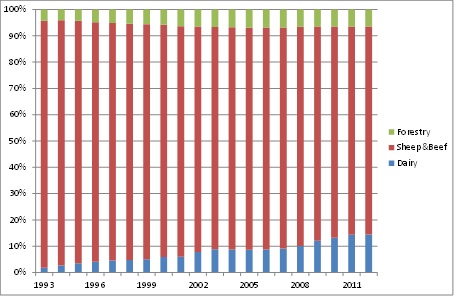
Figure 2. Historical land-use in Southland, major land-uses

4.2

To understand historical production trends, data on dairying farming operating revenue and expenditure were sourced from Dairy New Zealand, the country's main dairy industry group. Expenditure per hectare, income per hectare and prices remained relatively flat through the 1990s, with notable spikes in 2001 and 2008. In 1993, income and expenses were 40% of current levels; prices were about half. The production per hectare index exhibits a more constant growth trend over the last 20 years. In 1993, production per hectare was about 60% of the current level. These trends are shown in Figure 3. The figure presents indices for expenses per hectare, income per hectare, production per hectare and prices, all with the 2012 value set to 1.00.

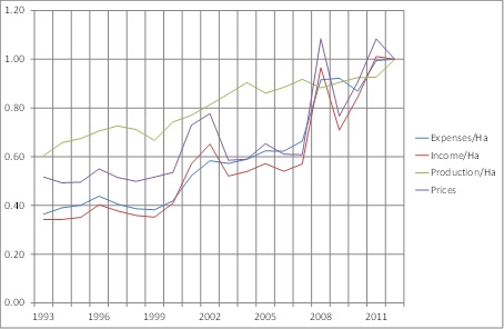
Figure 3. Historical dairy indices. Index (2012 = 1.00). Source: Dairy NZ, NZIER

4.3

Sheep and beef farming has had relatively flat returns over this period, as shown in Figure 4. In 1993, expenses per hectare and income per hectare were both about 60% of today's values. Prices were less than 45% of today. Production per hectare has remained fairly constant.

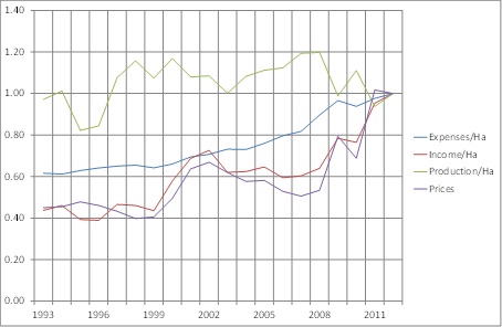
Figure 4. Historical sheep and beef indices. Index (2012 = 1.00). Source: Beef and Lamb NZ, Stats NZ, NZIER

4.4

An interesting comparison is the profitability of dairy versus sheep and beef, as shown in Figure 5. Sheep and beef profitability has increased slowly over time; dairy profitability has been more volatile, but significantly greater than sheep and beef at all times over the 20 year period. This is important when considering farmer decision-making. In every period, farmers concerned with maximising profits would compare sheep and beef farming to dairy farming and conclude that the latter was more profitable. A model of land-use change in Southland that relied solely on such economic calculations would tend to produce quick and significant land-use change. However, the fact that the actual trend has been a slow rate of conversion suggests that profit maximisation is not the sole driver of land use in Southland. For this reason, an agent-based model with decision rules other than profit maximisation was considered appropriate.

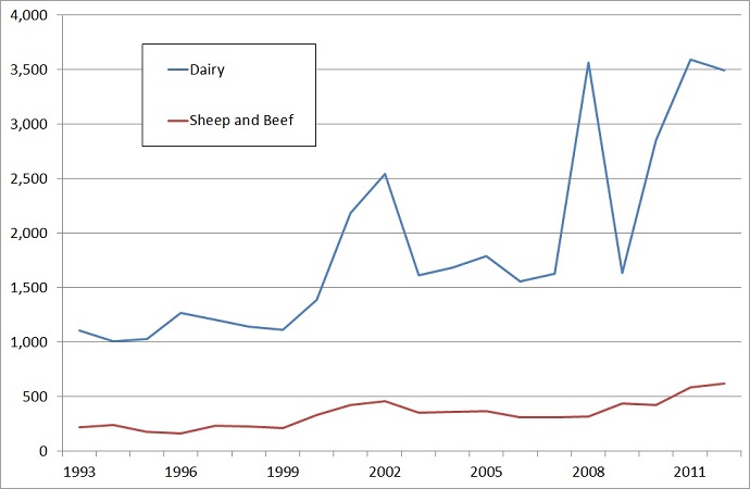
Figure 5. Profitability comparison. $/Hectare. Source: NZIER, Statistics NZ, Beef and Lamb NZ, Dairy NZ

Analysis

5.1

Dairy conversion in Southland has not had a steady rate of change. Instead, as shown in Figure 6, spikes in the milk solids price in 2001/2002 and 2008/2011 are associated with an increase in the rate of conversion of agricultural land into dairying, while the rate of conversion is lower before 2001 and between the spikes. This inconsistent rate of conversion in the face of a clear differential in returns to land uses was the focus of the validation. To validate the model, the goal was to reproduce the area in dairy farms as a percentage of agricultural land for every year in the dataset. Several parameters in the model have a direct bearing on land-use change. These parameters are described in Table 1. The validation method focused on the parameters about which there was the most uncertainty, and left unchanged the parameters for which there was more confidence about the values, which is the general lesson from Fagiolo et al. (2006).

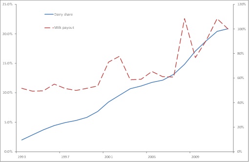
Figure 6. Price spikes and dairy conversions. LHS axis= dairy share of agricultural land in Southland. RHS axis = milk solids pay-out index (2012 = 100%). Source: NZIER, Dairy NZ, Statistics NZ, Beef and Lamb NZ

Table 1: Parameters affecting land use decisions
% peers	The higher the % of peers, the larger the peer group and the more likely a farmer was to observe a better farming outcome. Farmers must observe a better farming practice before they can adopt it. Higher % peers led to higher probability of change.
Comparison weighting factor	This factor described how much weight farmers put on information about the performance of different land uses. If weightings were all 1, then there was no difference between industries – farmers did not discount information they received from other land uses. If weightings were <1, then the parameter reduced the likelihood of change (like risk aversion). Higher weightings led to higher probability of change.
Median-time-to-change (inertia)	This median was a simple inertia parameter that reduced flip-flopping between land-uses. The higher the median-time-to-change, the lower the probability of change in any given year.
Maximum change a	This parameter provided the upper asymptote for the probability of change. A higher a increased the probability of change.
Minimum spike	The probability of change was related to levels but also to changes in levels, similar to the concept of a "just noticeable difference" (Gigerenzer & Selten 2001). This parameter was used to induce above-average land-use change. The higher this parameter, the less often a price increase is treated as a price spike leading to greater change.
Impact spike	This parameter adjusted the impact of a price spike on the probability of land-use change. The higher this parameter, the higher the probability of conversion when price spikes occur.

5.2

The bio-physical and economic rules were reasonably straight-forward and were validated by their theoretical strength (Berger et al. 2010). For example, dairying in Southland is on the whole confined to Land Use Capability classes 2 through 4. It is more difficult to run dairying operations easily and profitably on the higher numbered land classes, which have greater slopes and/or poorer-quality soils. Similarly, farm budgets are well understood: the profitability of dairying versus sheep and beef was based on Farmax modelling results, but was also supported by production budgets from the Ministry for Primary Industries and in Pangborn (2010). The comparison weighting factor was fixed at 0.75 and not changed for the calibration; the parameter is not used for the calibration exercise, but is available for future scenario development.

5.3

The median-time-to-change parameter was set at seven years. When used in the sigmoid probability of change equation (see Appendix B),

C = a − a/(1+exp(t−med)),

where C is the probability of change, a is the maximum change, t is the time since last change and med is the median time to change, the parameter produces a low probability of change in the first few years and a steeply rising probability in the next few years. It reach 95% of the maximum change probability a in year 10. Because the rate of conversion increased and decreased over time, a step was added to the basic decision algorithm (described in Appendix B). If prices in an industry spiked above a certain growth rate, the likelihood the farmer changing to that land use was increased. In mathematical terms, the algorithm was as follows:
If           p(t)/p(t-1) − 1 > minimum spike
then         C' = C* (1 + impact spike)
where
           p(t) = the commodity price in year t
           minimum spike = the price spike required to induce the additional behavioural response
           impact spike = the impact of the price spike on the probability of land-use change.
These two parameters were estimated by analysing the historical data on the impact of price spikes on the rates of conversion, which is an appropriate validation technique (Fagiolo et al. 2006; Macal 2013).

5.4

Less well understood were the two remaining parameters linked to land-use decisions. First, the impact of the size of peer networks was not understood. The size of peer networks for Southland famers was not known. Secondly, the willingness of farmers to change land use and behavioural responses to information was not known. Burton (2006 , 2009) has argued that farmers move between stages (or "typologies") over the life-course: risk-taking and profit-maximising in their early years of farming before typically becoming more risk-averse and cost-minimising as they near retirement. However, the link between these dynamics and actual farmer behaviour with respect to land-use change has not been readily quantified. The goal of the validation exercise was therefore to calibrate the maximum probability of change and percentage of peers parameters.

5.5

The analysis used a step-wise process to select likely values for the two parameters. First, the model was run using a range of values for the two variables. The results in the final year (2012) were compared with the actual share of dairying in Southland (16.6% of land area). Parameters that led to model results between 16% and 20% were retained for further inspection. Secondly, the year-by-year model results were compared against annual data for actual dairying area. Standard deviations were calculated by conducting 20 simulations for each set of parameters. The fit of the actual area to the averages and standard deviations was assessed visually, and likely central values for the two parameters were selected. Finally, sensitivity tests for the two parameters were conducted to confirm the selection of central estimates.

Results

Calibrating to land-use change

6.1

The result of the analysis is shown in Figure 7, which compares the share of dairying in Southland in RF-MAS in each time-step versus the actual growth in dairying over the last 20 years. The figure indicates that RF-MAS was able to replicate the growth in dairying. It was particularly accurate for the later years of the comparison as the share of dairying grew.

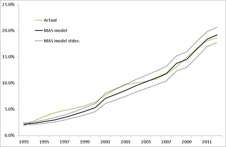
Figure 7. MAS model versus actual dairy conversion. Percentage area of agricultural land used for dairying

6.2

The result in Figure 7 is based on final calibrated values for the two studied parameters shown in Table 2. The percentage of peers was specified as a percentage of the total number of farmers in the geographic area being analysed. In this case it suggested each farmer had around 35 peers. The maximum change, which provided a maximum probability of a farm changing land use, was set at 3%. The goodness of fit can be calculated by comparing actual annual data to modelled data using a similar calculation to the coefficient of determination (R²) for regression models (Kennedy 2003, p. 29):

R2 = 1 − (error sum of squares / total sum of squares).

6.3

The goodness of fit of the simulation can similarly be estimated by dividing the error sum of squares from the model by the total sum of squares. The numerator is the sum over the period of the squared difference between the actual area and the modelled area. The denominator is the sum of the squared difference between the actual value for each year and the average for the period. For the parameter values in Table 2, the goodness of fit was 0.884.

Table 2: Parameter values
% peers	3%
Maximum change a	3%

6.4

The results for the two parameters were also subjected to sensitivity analysis to determine the impacts of the various decision parameters on final results.

Sensitivity test 1: Percentage of peers

6.5

The first sensitivity test compared the baseline of 3% peers to results from 2.5% and 3.5% peers. Figure 8 shows that changing the % peers parameter by 0.5% moved the results by about one standard deviation. It also suggests that the standard deviation increased as the % peers was reduced, indicating increased uncertainty around model results as the peer groups are restricted. In RF-MAS, information about land use is obtained from peers. With smaller peer groups, farmers have less information on alternative land uses available.

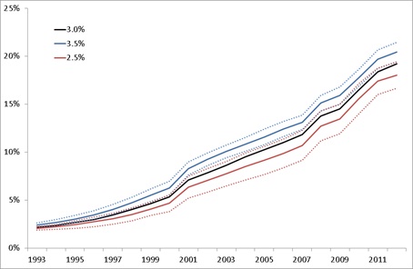
Figure 8. Sensitivity to percentage of peers Percentage area of agricultural land used for dairying

Sensitivity test 2: maximum change

6.6

In the second sensitivity test, the maximum change parameter was adjusted. The baseline was 3%, and values of 2% and 4% were also modelled. Figure 9 shows that changing the maximum change parameter by 1.0% moved the results by about one standard deviation. The standard deviation also increased as the maximum change parameter increased. Allowing for a greater possibility of change increased the uncertainty around farmers' choices of land use.

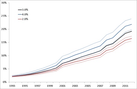
Figure 9. Sensitivity to maximum change. Percentage area of agricultural land used for dairying

Discussion

7.1

The research had the goal of validating a MAS model of rural Southland in New Zealand. The validation was intended to make the model useful for research on farming in Southland. The "right problem" to address (Macal 2013) was the expansion of dairying, a key element of land-use change and concern for the region. The validation therefore focused on reproducing the observed land-use change over the past 20 years.

7.2

The validation focused specifically on two themes from the literature on validation for simulation models. The first theme was scope. Following Galan et al. (2009), the research first determined the scope of the validation by identifying the important issues in Southland and validating the model around a key issue. In addition, policy makers and industry groups are interested in the process that leads to land-use change. Because changes at the farm level are the result of decisions by individual famers, RF-MAS particularly focused on those decisions.

7.3

The second theme from the literature was empirical validation, with reference especially to Fagiolo et al. (2006) and Schreinemachers and Berger (2011). The historical experience of conversion to dairying was taken as a phenomenon to be explained. The validity of RF-MAS was partly established by building the model based on sound theory, which provided indirect calibration. In addition, several elements of RF-MAS were set by reference to other data or modelling, such as the relative profitability of dairying and sheep and beef farming. Additional modelling on the historical data also provided estimates of some parameters. It was found, for example, that conversion did not happen smoothly over time, so the relationship between spikes in the commodity price of milk solids and increases in conversion rates were used to improve the model. Finally, RF-MAS was calibrated to historical land-use change data for the region by identifying key uncertain parameters, conducting multiple simulations, and selecting parameter values that provided good fit. The goodness of fit statistic between the historical data and the model results was 0.884, and sensitivity analysis showed that different values of the calibrated parameters led to worse fit. The results showed that RF-MAS could reproduce the history of land-use change in Southland, which is taken as validation of RF-MAS for the purpose of modelling land use by linking farmer decisions to regional trends.

7.4

The research is an example of a practical application of the theory of validation, providing some commentary on the validation literature. First, it demonstrates that meaningful validation is possible, despite some critics (Windrum et al. 2007). The validation reported here demonstrates that modellers can reproduce observed phenomena with some accuracy, provided they properly establish the scope of validation and focus on key areas of uncertainty. This validation can be "meaningful" by allowing researchers and others to understand the phenomena better. Secondly, it is an example of how validation can be done using the ideas from the theory of validation. Important elements are: using stylised facts to limit the parameter space ex ante, establishing the range of model outcomes and focusing on the most likely parameter space, focusing the search for parameter values where there is the greatest uncertainty, and using historical data to calibrate models.

7.5

One limitation of the exercise is the focus on a single model. The research validated a particular model by setting some parameters through theory, estimating other parameters separately through statistical analysis, and calibrating two parameters through simulation. A different model would likely produce different results. In particular, it might provide different estimates of the size of farmer peer groups and the maximum annual likelihood of changing land uses. One possible comparison is to the slow rate of dairy conversion reported by Kerr and Olssen (2012), although they focused on land-use changes at the national scale. With more work, additional external validation of model parameters may be possible.

7.6

Development of this particular model, RF-MAS, can proceed in a few directions. One direction is scenario modelling of Southland using the existing model. The model is now a tool that researchers and community members can use to explore "what-if" questions and think about potential futures for the region. A second direction is towards greater generalizability. The model is based on data specific to Southland and calibration to historical trends in Southland. There is therefore the potential for overfitting: the model may explain the past very well without providing a good guide to the future. To examine the potential impacts of overfitting, RF- MAS can be applied to other regions of New Zealand. A third direction is towards more detail and specificity. In particular, the behaviour of farmer-agents in the model – reliance on peer networks, propensity to change, and other behaviour elements – can be explored and improved.

Acknowledgements

This work was funded by the New Zealand Foundation for Research, Science and Technology and AgResearch Limited through the Rural Futures programme.

Appendix A

8.1

RF-MAS is a file written in C# that calls data from CSV files and produces output in the same format. The process of the model is shown in a series of figures.

8.2

The first figure is the Initialisation phase. This phase obtains data about the farms and farmers to be modelled, links one farm to one farmer, and create social networks of farmers.

8.3

The next three figures concern each time-step of the model. Each time-step has three phases: Pre-processing, Main processing, and Post-processing. The Pre-processing phase is focused on ageing farmers by one year and updating any related information, such as their economic objective and risk behaviour. In the Main processing phase, farmers make a choice about the land use on their farms. They do this by determining whether to change their land use, and then selecting the land use that best meets their objectives. The Post-processing phase updates the farm accounts, calculates economic performance, calculates nutrient losses, and handles farmer retirement. The model then returns to the Pre-processing phase and goes through the next time step or terminates.

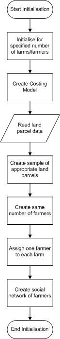
Figure A1. RF-MAS Initialisation phase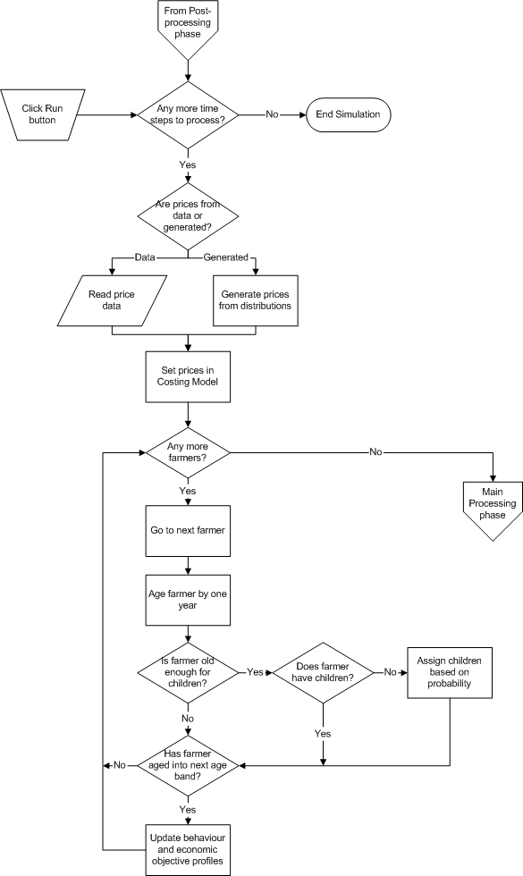

Figure A2. RF-MAS Pre-processing phase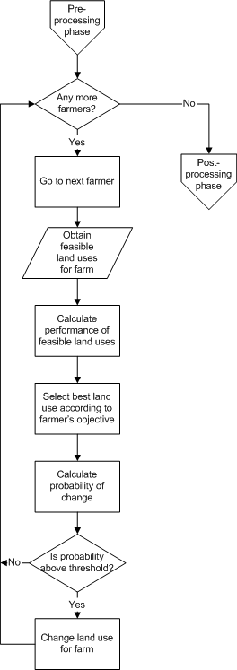

Figure A3. RF-MAS Main processing phase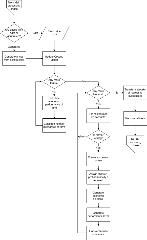

Figure A4. RF-MAS Post-processing phase

Appendix B

9.1

RF-MAS is described using the updated 'ODD' (Overview, Design concepts, and Details) protocol (Grimm et al. 2010). Elements of the ODD protocol that are not relevant are excluded.

Purpose

9.2

The MAS is intended to investigate future impacts of multiple pressures on rural communities through their impacts on the New Zealand pastoral industry. These pressures include market, societal and policy changes that operate at local, national and international scales, as well as resource issues such as energy costs, water availability and labour shortages. The intended audience is policy makers, farm advisors and industry personnel.

9.3

The MAS has two purposes: communication and analysis. The two modes of use, Web and desktop, correspond roughly to those two purposes. The Web model uses a visually appealing, interactive user interface. An experienced user can guide non-users through the input data and display selected outputs, enabling non-users to be involved in running the model. This mode therefore enables communication between researchers and stakeholders: stakeholders can suggest input value or model scenarios to test, and researchers can demonstrate the impacts of assumptions and future pressures on the pastoral sector. The desktop mode is designed for use in analysis, allowing batch processing of multiple scenarios and multiple simulations of a single scenario, and also allowing greater control over parameter values and distributions. Both modes use the same engine and input file structure, but with different user interfaces and different presentation of output data.

Entities, state variables and scales

Agents

9.4

There is only one type of agent in the model: farmers. Farmers are described by their age, presence of successor and initial industry. Age, successor and initial industry are assigned probabilistically based on distributions from existing data, including the Agribase database of farms in New Zealand.

Land/farms

9.5

Data on land/farms are sourced from Agribase and the Land Resources Inventory (LRI). A farm is described by its GIS coordinates and assigned a score based on the productivity-weighted average Land Use Capability (Lynn et al. 2009) class of all the parcels on the farm. Farms under 20 hectares are excluded. Farms suitable for dairying are identified based on size and LUC score; such farms are able to be used for dairying, although they may actually have other land uses. There are over 3000 farms in the Southland land database.

Process overview and scheduling

9.6

The model has three 'layers': land, land use, and farmer/agent. Initially, agents and land parcels are assigned to each other and the use of the land is determined. The land use includes the industry (e.g., sheep and beef, dairying), the intensity of the activity (as given by stocking rate), and activities to mitigate the environmental impacts of farming. At the end of each time-step, the economic and environmental performance of each farm is determined, and a propensity to change is calculated for each agent. An agent surveys the network of peers to determine which one is doing best, and then 'decides' whether to imitate the activity of that peer.

9.7

The engine of the MAS is a C# file that gathers inputs, processes, and generates outputs. This file is largely independent of the input data, with the exception of some variable naming that is currently coded in the engine. The land data is read into the model from a comma-separated file (CSV) file of Geographical Information System (GIS) data describing land parcels to be used for farms. Data for land use, including stocking rates, nutrient losses, farm costs and more, are contained in spreadsheet (XLS) files. An XML file contains data used to synthesise the farmer agents and additional local and national social, economic and financial data; this file is used to describe a particular scenario.

9.8

Each time-step represents a year. There are three stages in each step of a simulation:

• Before the time-step, adjustments are made to agent ages and presence of children, which can lead to changes in economic objective
• During the time-step, each farmer observes network peers are and decides whether to change land use
• After the time-step, prices and costs are updated, farm performance is calculated, and any retiring farmers are replaced.

Design concepts

Basic principles

9.9

The basic principle is that the farm/agent dyad is central to MAS. All data – biophysical, social, economic – need to relate to either the farmer or the farm, i.e., the person or the land. The agent makes the decision on land use according to the information available, constrained by the capability of the specific land parcel. Policies and pressures need to be linked to agent, land use, or land. For example, specific land uses can be mandated or proscribed on certain types of land. All inputs and outputs are specified at the farm level, although they may be derived from per-hectare data. All activities happen on an annual basis, in keeping with the one-year time-step.

Emergence

9.10

Emergence in MAS models arises from interactions amongst the agents (Tesfatsion & Judd 2006). In this MAS, farmer-agent interaction is via peer networks. Agents learn which land uses are successful by observing peers in their networks having success. Adoption of new farm practices or technologies is an emergent property of the system. Adoption happens more or less quickly depending on the amount of information available, the extent of peer networks, the objectives of agents and the fit of innovations with the capabilities of the land.

Adaptation

9.11

Agents adapt to new conditions without foresight and with little information about the past. In order to change, each agent must both decide to change land use (a probabilistic occurrence in the model) and observe a peer having more success at some other land use (which is a function of the size and composition of peer networks). Agents use information on own performance and peer performance only from the year they make the decision to change land use.

9.12

Upon observing a peer with a preferable result, the agent needs to decide whether to change land use to match that of the peer. This decision is based on the risk-aversion of the farmer (which in turn is based on their age and presence of a successor) and a median-time-to-change parameter, in a function that creates a sigmoid curve. The probability of change C, is calculated by following function:

C = a - a/(1+exp(t-med))

where
C = probability of acting on observation and changing land use
t = time since last change
med = median-time-to-change
a = maximum change
The second term is an inertia term that restricts farmers from constantly changing land use. The exponential function uses that actual time since last change and the median-time-to-change parameter to adjust the probability of change. At the median time, the probability of change is one-half the maximum change. The larger the median, the stronger is the inertia for the farmer to stay in their current land use and not change. The maximum change parameter a, imposes a limit on the likelihood of change. The reason for this limit is to account for farmers who do not want to change land use, regardless of time since a previous change.

Objectives

9.13

Agents have one of three objectives. They are: profit maximisation, production maximisation with low inertia and cost minimisation. An agent's objective is assigned probabilistically at model initialisation and when the agent moves into a new age bracket. The probability of one of the three objectives is conditional on age and presence of successor, based on Burton (2009). Cost minimisation simulates farmers who are seeking to reduce the demands of the farm on their time, perhaps as a prelude to retiring altogether.

Learning

9.14

Agents have information available to them through their peer networks. Agents do not, however, accumulate knowledge or information themselves.

Prediction

9.15

Agents are myopic about the future; there is no forward-looking component to their decisions.

Sensing

9.16

Agents are able to know their own performance, including their financial performance and their environmental performance. They are also able to know the financial and economic performance of their peers. The MAS includes a comparison weighting parameter, which has agents 'discount' the information they receive from peers outside their industry group.

Interaction

9.17

Agents interact with each other once per year, when they reveal information about economic and environmental performance to each other. Agents do not, however, give advice to peers, direct them or negotiate with them.

Stochasticity

9.18

The MAS has the ability to include stochastic prices for inputs and outputs, such as nitrogen and fuel prices (inputs) and milk and meat prices (outputs). The type of distribution can be specified, such as Normal or triangular, and the size of the deviation can also be specified. Quantities of outputs are not stochastic, and neither are the environmental parameters.

Collectives

9.19

An agent is given a percentage of farmers for a peer network, which percentage can be adjusted. First, two sets or 'pools' of farmers are created. For one pool, farmers are put into two age-defined sub-pools, those younger than 45 and those 45 and older. In the second pool, farmers are divided into sub-pools according to their current industry. Each farmer is both in an age sub-pool and an industry sub-pool. The network library then creates networks of peers within each of these sub-pools so that each farmer knows the set percentage of other farmers in the same pool (i.e. within the same age-group and within same industry). These networks are then merged so that each farmer ends up with a network of peers, with some in the same age-group and some in the same industry (and some both). The networks are based on the Erdös–Rényi model.

Initialisation

9.20

Initialisation of a model scenario progresses through the following steps:

• Input data are read
• Agent farmers are created using the appropriate distributions of age, presence of children, economic objective and ability
• Agents are allocated into peer groups based on age and industry
• Farms are created according to the initial percentage industry mix, if they have not been read in from the land data file
• Farms are allocated to farmers (in the case of synthetic farms) or farmers are allocated to farms (if land use is part of the land data file)
• Part of the first time-step is creating the financial accounts for the farm and agent, which include income, assets and liabilities

Inputs

9.21

There are two sets of inputs to the model:

• Production and nutrient budgets for land uses
• Prices for inputs and outputs.

Land uses are described by production and nutrient budgets. Each farm has a set of potential land uses from which the farmer-agent can choose. This set is determined by characteristics of the land, such as Land Use Capability class and soil drainage. It may also be restricted by policy, such as a policy that limits nitrogen leaching to a specified cap. Production budgets are estimated for different types of land using Farmax and Apsim models, and include data on production costs, productivity and profits. Nutrient budgets are estimated using the Overseer model (version 6), and include data on nitrogen and phosphorus losses. Considering the four different mitigation possibilities, the three levels of production intensity and the two pastoral industries, up to 24 pastoral agricultural budgets and one forestry budget are available for any single farm. A total of 121 production and nutrient budgets were estimated for the six types of land, being three land productivity classes and two drainage classes.

9.22

The second set of inputs is prices for input costs and commodities produced. They can be set as levels or trends, or entered as vectors of prices for the entire time period of the model.

Submodels

9.23

The MAS does not contain any submodels. It is, however, informed by modelling from Farmax, Apsim and Overseer, as described above.

Appendix C

This appendix contains class diagrams for key elements of RF-MAS. Note that RF-MAS is a continuing project, so that the class diagrams contain elements that are not currently used.

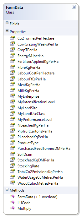
Figure C1. Farm class diagram for RF-MAS

Figure C2. FarmData class diagram for RF-MAS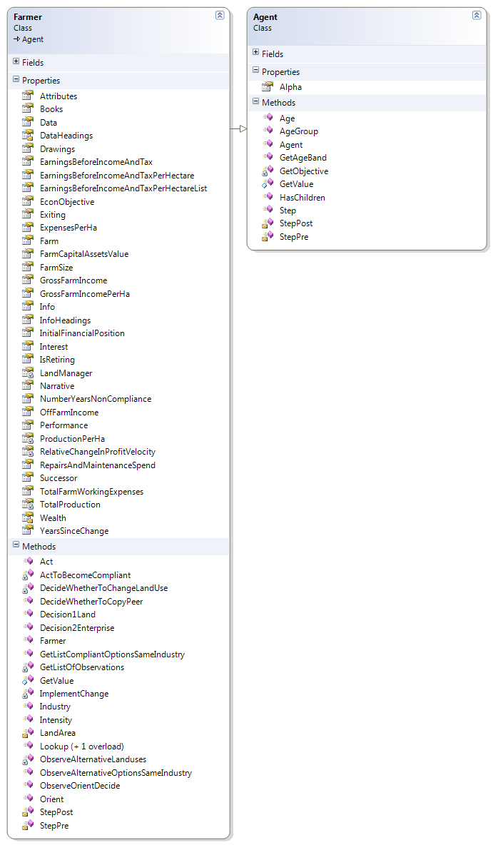

Figure C3. Farmer-Agent class diagram for RF-MAS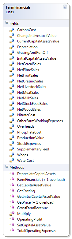

Figure C4. FarmFinancials diagram for RF-MAS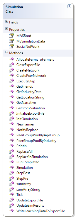

Figure C5. Simulation class diagram for RF-MAS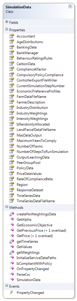

Figure C6. SimulationData class diagram for RF-MAS

References

ASUREQUALITY NEW ZEALAND. (several years). AgriBase Database. Retrieved from http://www.asurequality.com/capturing-information-technology-across-the-supply-chain/agribase-database-for-nz-rural-properties.cfm

AUGUSIAK, J., Van den Brink, P. J., & Grimm, V. (2014). Merging validation and evaluation of ecological models to "evaludation": A review of terminology and a practical approach. Ecological Modelling, 280, 117–128. [doi:10.1016/j.ecolmodel.2013.11.009]

BELL, A. R. (2011). Environmental licensing and land aggregation: an agent-based approach to understanding ranching and land use in rural Rondônia. Ecology and Society, 16(1), 31.

BERGER, T., Birner, R., Diaz, J., McCarthy, N., & Wittmer, H. (2007). Capturing the complexity of water uses and water users within a multi-agent framework. Water Resources Management, 21, 129–148. [doi:10.1007/s11269-006-9045-z]

BERGER, T., Schilling, C., Troost, C., & Latynskiy, E. (2010). Knowledge-Brokering with Agent-Based Models: Some Experiences from Irrigation-Related Research in Chile. International Environmental Modelling and Software Society (iEMSs) 2010 International Congress on Environmental Modelling and Software Modelling for Environment's Sake, Fifth Biennial Meeting, Ottawa, Canada. Retrieved from http://www.iemss.org/iemss2010/papers/S07/S.07.12.Knowledge%20Brokering%20with%20AgentBased%20Models%20%20Some%20Experiences%20from%20Irrigation%20Related%20Research%20in%20Chile%20-%20THOMAS%20BERGER.pdf

BHARATHY, G. K., & Silverman, B. G. (2010). Validating agent based social systems models. In Proceedings of the 2010 Winter Simulation Conference (pp. 441–453). IEEE. Retrieved from http://repository.upenn.edu/cgi/viewcontent.cgi?article=1630&context=ese_papers [doi:10.1109/WSC.2010.5679142]

BURTON, R. (2006). An alternative to farmer age as an indicator of life-cycle stage: the case for a farm family age index. Journal of Rural Studies, 22 (4), 485-492. BURTON, R. (2009). Strategic decision-making in agriculture: an international perspective of key social and structural influences. Report (unpublished) to the Rural Futures programme, Agresearch, New Zealand

FAGIOLO, G., Windrum, P., & Moneta, A. (2006). A critical guide to empirical validation of agent-based economics models: methodologies, procedures, and open problems (No. 2006-14).

GALAN, J. M., Izquierdo, L. R., Segismundo S. Izquierdo, José Ignacio Santos, Ricardo del Olmo, Adolfo López-Paredes, & Bruce Edmonds. (2009). Errors and Artefacts in Agent-Based Modelling, Journal of Artificial Societies and Social Simulation,12(1), 1. https://www.jasss.org/12/1/1.html

GIGERENZER, G., & Selten, R. (Eds.). (2001). Bounded rationality: the adaptive toolbox. Cambridge, MA: MIT Press.

GRIMM, V., Berger, U., DeAngelis, D. L., Polhill, J. G., Giske, J., & Railsback, S. F. (2010). The ODD protocol: A review and first update. Ecological Modelling, 221(23), 2760–2768. [doi:10.1016/j.ecolmodel.2010.08.019]

HERSPERGER, A. M., Gennaio, M., Verburg, P. H., & Bürgi, M. (2010). Linking land change with driving forces and actors: four conceptual models. Ecology and Society, 15(4), 1.

JIN, E., Girvan, M., & Newman, M. (2001). Structure of growing social networks. Physical Review E, 64(4). [doi:10.1103/PhysRevE.64.046132]

KAYE-BLAKE, W., Li, F. Y., Martin, A. M., McDermott, A., Rains, S., Sinclair, S., & Kira, A. (2010). Multi-agent simulation models in agriculture: a review of their construction and uses (Research Report No. 318). Lincoln, N.Z.: Agribusiness and Economics Research Unit (AERU), Lincoln University.

KENNEDY, P. (2003). A guide to econometrics. Cambridge, Mass.: MIT Press.

KERR, S., & Olssen, A. (2012). Gradual land-use change in New Zealand: results from a dynamic econometric model. Motu Economic and Public Policy Research. Retrieved from http://motu-www.motu.org.nz/wpapers/12_06.pdf [doi:10.2139/ssrn.2061389]

KLÜGL, F. (2008). A validation methodology for agent-based simulations. In Proceedings of the 2008 ACM Symposium on Applied Computing (pp. 39–43). New York, NY, USA: ACM. [doi:10.1145/1363686.1363696]

LAND RESOURCE INVENTORY AND LAND COVER DATABASE. (2012). Retrieved from https://lris.scinfo.org.nz/.

LYNN, I., Manderson, A., Page, M., Harmsworth, G., Eyles, G., Douglas, G., … Newsome, P. (2009). Land Use Capability Survey Handbook (3rd ed.). Hamilton: AgResearch; Lincoln: Landcare Research; Lower Hutt: GNS Science.

MACAL, C. M. (2013, May 7). On validating multi-agent system applications. Keynote Address MABS 2013 presented at the 14th International Workshop on Multi-Agent-Based Simulation, Saint Paul, Minnesota, USA. Retrieved from http://www2.econ.iastate.edu/tesfatsi/MASValidation.Macal2013.pdf

MCCARL, B.A., & Apland, J.D. (1986). Validation of linear programming models. Southern Journal of Agricultural Economics, 68(5), 155-164.

MARKS, R. E. (2013). Tutorial: validating simulation models, and multi-agent systems in the social sciences. CIFEr Singapore (p. 75 p.).

MILLINGTON, J. D. A., Demeritt, D., & Romero-Calcerrada, R. (2011). Participatory evaluation of agent-based land-use models. Journal of Land Use Science, 6(2–3), 195–210. [doi:10.1080/1747423X.2011.558595]

MOSS, S. (2008). Alternative approaches to the empirical validation of agent-based models. Journal of Artificial Societies and Social Simulation, 11(1), 5. https://www.jasss.org/11/1/5.html

PANGBORN, J. (Ed.). (2010). Financial budget manual 2010. Lincoln, N.Z.: Lincoln University.

RABIN, M. (2002). A perspective on psychology and economics. European Economic Review, 46(4–5), 657–685. [doi:10.1016/S0014-2921(01)00207-0]

RICHIARDI, M., Leombruni, R., Saam, N., & Sonnessa, M. (2006). A common protocol for agent-based social simulation. Journal of Artificial Societies and Social Simulation, 9(1), 15. https://www.jasss.org/9/1/15.html

SCHREINEMACHERS, P., & Berger, T. (2011). An agent-based simulation model of human–environment interactions in agricultural systems. Environmental Modelling & Software, 26(7), 845–859. [doi:10.1016/j.envsoft.2011.02.004]

SIMON, H. A. (1955). A behavioral model of rational choice. Quarterly Journal of Economics, 69(1), 99–118. [doi:10.2307/1884852]

TESFATSION, L., & Judd, K. L., eds. (2006). Handbook of Computational Economics, Vol. 2: Agent-Based Computational Economics. Handbooks in Economics Series. North Holland, Amsterdam: Elsevier.

VILLAMOR, G. B., van Noordwijk, M., Troitzsch, K. G., & Vlek, P. G. (2012). Human decision making for empirical agent-based models: construction and validation (p. [8] p.). Presented at the International Environmental Modelling and Software Society (iEMSs) 2012 International Congress on Environmental Modelling and Software Managing Resources of a Limited Planet, Sixth Biennial Meeting, Leipzig, German, International Environmental Modelling and Software Society (iEMSs). Retrieved from http://www.zef.de/module/register/media/21fd_Villamor_et%20al_%20decision%20making.pdf

WINDRUM, P., Fagiolo, G., & Moneta, A. (2007). Empirical validation of agent-based models: alternatives and prospects. Journal of Artificial Societies and Social Simulation, 10(2), 8. https://www.jasss.org/10/2/8.html