
Introduction
Social conventions play decisive roles in everyday life. These rules of conduct assist in social interactions by prescribing the choice of one particular alternative if several are available. Examples are the rule of right- or left -hand driving in a country, the way of greeting among members of a cultural group, or the usage of the same software in a company. In either case, multiple alternatives are feasible, but the agreement on one alternative is advantageous. Therefore, conventions differ from other social norms by being self-preserving once they are established. Compliance is sought by everyone because of an automatic punishment after deviation.
A more complicated issue in the explanation of social conventions is their initiation. Schelling (1960) addressed this difficulty in his study of social conflict. Due to limited communication and perception, the initial agreement on a behaviour can be problematic although the common behaviour is in everyone’s best interest (Schelling 1960, p. 84). In any situation without central authority, the actors must coordinate their choices, and the outcome depends on the available information and the actors’ way of decision-making. Hence, the main question in the study of social conventions concerns their establishment.
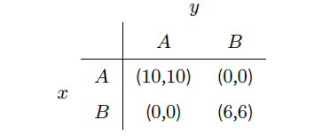 |
Following the work of Schelling, the evolution of social conventions has usually been modelled by n-way coordination games (e.g. Young 1998). These games refer to the sequential play of two-person coordination games with multiple partners. A sample two-person coordination game is shown by Table 1. The two actors, which are denoted by x and y, must decide between alternatives A and B. Given a pair of decisions, the table defines the rewards. Nothing is gained in case that actors choose different alternatives. If both actors take the same alternative A or B, they receive a reward of 10 or 6, respectively.
Given an n-way coordination game, a social convention is said to be established if all actors agree on one alternative. Young (1993) analysed these games in case of random actor matching. At each round of the game, two actors were randomly drawn from a large population. Both actors knew the reward structure of the stage game, and decisions were made by selecting an alternative with the highest expected reward given some information about previous interactions. As result, Young (1993) found that actors learn to establish a convention and, more specifically, play a risk-dominant equilibrium of the stage game (see also Kandori et al. 1993). The concept of risk-dominance takes into account that, if the partner’s decision is not known with certainty, one action may be less risky than another one (Harsanyi & Selten 1992, pp. 82-84). For example, the game of Table 1 has two pure Nash equilibria (A; A) and (B; B) with the former being risk-dominant. Risk-dominance is not necessarily equivalent to efficiency, which denotes the equilibrium with the highest rewards (see game II of Table 2).
In addition to random matching, Young (1998, ch. 6) also considered n-way games in networks. In any larger group, interaction between members is limited. Every actor has a small group of partners with whom he/she interacts. Additionally, information about previous encounters is restricted to this group. Similar to the model with random interactions, the analysis of Young (1998, ch. 6) indicated that only risk-dominant equilibria are stable, and all members of a connected component[1] of the network eventually choose the same alternative.
In other words, the network structure had no effect on the outcome of the n-way game. This result was due to random mistakes, which the actors made with strictly positive probability. Without mistakes, the network structure affects the outcome (Buskens & Snijders 2016), and also risk-dominated equilibria occur. Furthermore, it is possible that two different conventions coexist in some networks (see also Berninghaus & Schwalbe 1996).
Overall, the results suggest that the particular combination of behavioural assumptions and network structure is relevant. In regard to behavioural assumptions, the models of all previously mentioned studies can be characterised as “myopic best reply” (Berninghaus & Schwalbe 1996, p. 300). Given this model, actors learn about the partners’ behaviour from past interactions and use this knowledge to choose a best action given the reward structure of the game. This means that information about the situation and past actions of the partners was presumed to be available in all former studies.
While these are reasonable assumptions in most situations, this paper asks about the theoretical implications of dropping them: Is it possible to explain the emergence of conventions if actors are neither aware of the payoff structure nor the choices of other actors. The contribution of this paper is, thus, mainly theoretical, but with relevance to future empirical research. For instance, in case that the results differ from previous studies, conclusions can be drawn from empirical macro-level observations to micro-level assumptions.
A behavioural model in which an actor’s decision is based only on her own previous actions and rewards is called completely uncoupled (e.g. Babichenko 2012). Despite this limiting setting, some learning models still ensure the convergence of behaviour to Nash equilibria (Foster & Young 2006; Germano & Lugosi 2007; Young 2009; Babichenko 2012). For example, Pradelski & Young (2012) introduced a model of completely uncoupled learning that yields welfare-maximising Nash equilibria in two-person coordination games.
However, the behavioural model of Pradelski & Young (2012) was designed to converge to equilibria. The assumptions were not justified by empirical observations or psychological experiments. In contrast, most psychological models of learning were developed to represent the development of human behaviour as realistic as possible (e.g. Staddon 2001). Some popular instances of realistic models implement a form of learning known as operant conditioning or reinforcement learning (Sutton & Barto 1998; Staddon & Cerutti 2003). These models are completely uncoupled but do not necessarily converge to an equilibrium in interactive situations.
In this paper, a simple and empirically grounded model of reinforcement learning is used to analyse the behaviour in n-way coordination games. Following past research, this model is called melioration learning. The details are given in the next section. Afterwards, it is shown that actors who learn by melioration are able to coordinate their decisions in n-way coordination games and, hence, to establish a convention. The long-term outcome is a risk-dominant equilibrium of the two-person stage game if one exists. The results are compared to the predictions of another, well-known model of reinforcement learning: the Roth-Erev model (Roth & Erev 1995). While the outcomes are qualitatively similar, the models differ in their speed of convergence, especially in regard to the effects of the network structure.
Melioration learning
Given a situation of repeated decision-making, melioration learning states that a behaviour is strengthened if it comes with the currently highest average value. The theory was introduced by Herrnstein & Vaughan (1980) in order to explain a widely observed empirical regularity known as the matching law (Baum 1979; Pierce & Epling 1983; McDowell 1988; Herrnstein 1997; Vollmer & Bourret 2000; Borrero et al. 2007). The predictions of melioration learning were tested and confirmed in numerous psychological experiments (e.g. Vaughan 1981; Mazur 1981; Herrnstein et al. 1993; Antonides & Maital 2002; Tunney & Shanks 2002; Neth et al. 2005).
The model
Unlike previous formal representations of melioration (Brenner & Witt 2003; Sakai et al. 2006; Loewenstein 2010), this paper uses a model that is perfectly consistent with the ideas of Vaughan & Herrnstein (1987) and builds on an algorithm of decision-making that is called \(\varepsilon\)-greedy strategy (Sutton & Barto 1998, p. 28). This strategy takes a parameter \(\varepsilon \in (0,1)\), which is called exploration rate and specifies the probability of an alternative being chosen uniformly at random. With probability \(1-\varepsilon\), an alternative with the currently highest value is selected. If multiple alternatives have the highest value, one of them is chosen randomly. In melioration learning, the value of an alternative is the average of the corresponding past rewards.
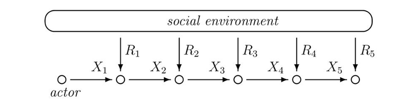
Figure 1 illustrates the decision-making process, which takes place along discrete time steps \(t \in \mathbb{N}\). Given a finite set of choice alternatives \(E\), actions are emitted by the choice of an element \(X_t \in E\) from the set of alternatives. After every decision, a non-negative reward \(R_{t} \in (0,\infty)\) is received from the environment and processed by the actor. The information processing is very simple and specified by algorithm 1.
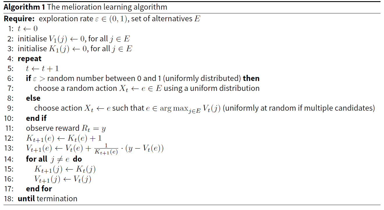
In algorithm 1, an actor is assumed to maintain a set of values \(\left\lbrace V_{t}(j) \right\rbrace_{j \in E}\) that are iteratively updated. Initially, all values are set to zero. A set of frequencies \(\left\lbrace K_{t}(j) \right\rbrace_{j \in E}\) keeps track of the number of choices of each alternative. The reward realisation \(y = R_{t}\) is used to modify the value of the chosen alternative such that it gives the average of all past rewards of \(e\).
Comparison with other models of learning
In economics, Brenner (2006) distinguished two types of learning: reinforcement learning and belief learning (a similar categorisation is found in Camerer 2003, ch. 6). Melioration is categorised as reinforcement learning because it is less cognitively demanding than belief learning models. The differences are elaborated in the following. Additionally, a comparison with other models of reinforcement learning is given.
Belief learning models
In algorithm 1, an actor learns the value of an alternative, which constitutes a belief about the environment. Since the actor responds to these beliefs in an optimal way, melioration learning can be seen as a rudimentary form of belief learning. However, melioration learning is different from most belief learning models. In the latter, the formation of beliefs generally exceeds the level of actions. Instead, the values of actions are externally given, and beliefs about the reinforcement mechanism or the behaviour of other actors are acquired. For example, in a two-person game-theoretic situation, the actors may know the structure of the game and learn the strategy of the opponent. A general belief learning algorithm for this situation is given by the following pseudocode (Shoham & Leyton-Brown 2009, p. 196):
Reinforcement learning models
Unlike belief learning, reinforcement learning is a simple idea about behavioural change. It can be summarised by Thorndike’s law of effect: "pleasure stamps in, pain stamps out". More specifically, behaviour that is followed by a positive experience is likely to reoccur, but, if provoking negative reactions, it diminishes over time. Two examples of reinforcement learning are the Bush-Mosteller and the Roth-Erev model.
The Bush-Mosteller model (Bush & Mosteller 1964) states that a probability of choice changes linearly in the level of satisfaction. More specifically, an actor chooses an element \(e \in E\) at time \(t \in \mathbb{N}\) with probability \(q_e(t) \in [0,1]\). After receiving a reward \(y_t \in \mathbb{R}\) for choosing \(e\), the probability is updated by
| $$q_e(t) = q_e(t - 1) + \left\lbrace \begin{array}{ll} (1 - q_e(t - 1)) \cdot \sigma(y_{t}) & \text{if } \sigma(y_{t}) \geq 0\\ q_e(t - 1) \cdot \sigma(y_{t}) & \text{if } \sigma(y_{t}) < 0\\ \end{array} \right.$$ | (1) |
The dynamics of Bush-Mosteller learning differ from the dynamics of melioration. This is seen when comparing the probabilities of choosing an action. According to algorithm 1, the probability of choosing \(e\) at time \(t\) is:
| $$\begin{array}{ll} \frac{1 - \varepsilon}{\left\vert{argmax_{j \in E} V_{t}(j)}\right\vert} + \frac{\varepsilon}{\left\vert{E}\right\vert}, & \text{if } e \in argmax_{j \in E} V_{t}(j), \text{ and }\\ \frac{\varepsilon}{\left\vert{E}\right\vert}, & \text{if } e \notin argmax_{j \in E} V_{t}(j).\\ \end{array}.$$ | (2) |
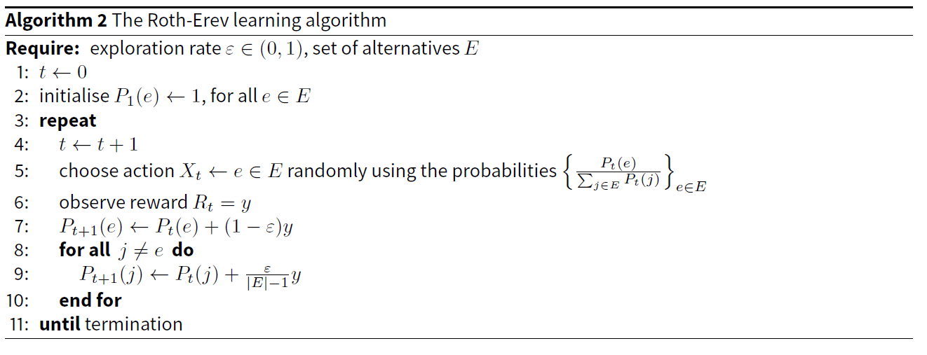
The Roth-Erev model describes another form of reinforcement learning and is widely known in economics. Algorithm 2 specifies its basic version (Roth & Erev 1995, p. 172). Instead of average values, the actor holds a set of accumulated values \(\{P_t(e)\}_{e \in E}\), which are called propensities. At each time step, an alternative \(e \in E\) is chosen with probability \(\frac{P_t(e)}{\sum_{j \in E} P_t(j)}\). The parameter \(\varepsilon\) maintains a level of exploration.
In the following analysis, the outcomes of melioration learning are compared to the predictions of the Roth-Erev model. In contrast to other learning processes, Roth-Erev is very similar to melioration. Both models take a "mechanistic perspective on learning", which means that “people are assumed to learn according to fixed mechanisms or routines” (Brenner 2006, p. 903). Additionally, simple versions with only one parameter (the exploration rate) exist. Other models of reinforcement learning, such as Bush-Mosteller, require additional assumptions or the specification of further parameters.
Bush-Mosteller and Roth-Erev are just two of many forms of reinforcement learning. Other models are, for example, developed and analysed by computer scientists in a field called RL (Sutton & Barto 1998). While these models differ from the ones in economics (Izquierdo & Izquierdo 2012), most of them are completely uncoupled as defined above. Moreover, melioration learning, as given by algorithm 1, constitutes a relatively trivial instance of an RL method that is called Q-learning (Watkins 1989). However, unlike the general version of Q-learning, melioration neglects any possible consequences of present actions on future rewards.
As pointed out at the beginning, melioration learning accounts for empirical observations in situations of repeated choice (see also Sakai et al. 2006, p. 1092). However, generally, there is “tremendous heterogeneity in reports on human operant learning” (Shteingart & Loewenstein 2014, p. 94). In particular, melioration seems too simple to accurately represent the complexity of human decision-making (e.g. Barto et al. 1990, p. 593) and more sophisticated models of learning have been suggested (e.g. Sutton & Barto 1998; Sakai et al. 2006). Nevertheless, it may serve as valid micro-level model in the study of social phenomena.
Analysis
Given that melioration leaning is implemented as instance of the \(\varepsilon\)-greedy algorithm with Q-learning, results from previous research can be adopted. On the one hand, algorithm 1 converges to optimal behaviour under certain assumptions of stationarity (Watkins & Dayan 1992). These situations include Markov decision processes (Bellman 1957) and, therefore, many non-social settings. Besides stationarity, convergence also requires that the exploration rate decreases sufficiently slowly towards zero, e.g. if a time-dependent exploration rate \(\varepsilon_t := \frac{\varepsilon}{1 + \sum_{j \in E} K_t(j)}\) instead of \(\varepsilon\) is used in line 6 of algorithm 1 (Jaakkola et al. 1994)
On the other hand, convergence is not guaranteed if multiple persons interact and reinforcements are contingent upon the decisions of everyone (Nowé et al. 2012, p. 451). While equilibria are reached in some two-person games (Sandholm & Crites 1995; Claus & Boutilier 1998; Gomes & Kowalczyk 2009), the behaviour fails to converge in general (Wunder et al. 2010). Moreover, there is no work about the convergence of Q-learning (and, thus, melioration learning) in situations with more than two actors. Because of the complexity of these situations, the convergence of any learning process is difficult to derive analytically.
In particular, a Markov chain (MC) analysis of the model (e.g. Izquierdo et al. 2009; Banisch 2016) is impeded by the adjustment of the values \(\left\lbrace V_{t}(j) \right\rbrace_{j \in E}\) as historical averages. In order to obtain a time-homogeneous Markov chain, each state must contain the sets \(\left\lbrace V_{t}(j) \right\rbrace_{j \in E}\) and \(\left\lbrace K_{t}(j) \right\rbrace_{j \in E}\) of all actors. The resulting chain is not irreducible because the frequencies \(K_{t}(j)\) cannot decrease with time. Only a time-inhomogeneous MC may be irreducible. However, either approach precludes the application of standard techniques. Fortunately, computer simulations can still be employed to analyse the model and derive hypotheses for particular situations.
In the following simulations, algorithm 1 (melioration learning) and algorithm 2 (Roth-Erev) are applied to n-way coordination games. In both cases, the exploration rate is set to \(\varepsilon = 0.1\) and kept constant during the whole simulation. This strictly positive rate allows a trade-off between the exploitation of the currently best action and the exploration of alternatives. Because of the finite nature of every simulation run, a continuously decreasing exploration rate would actually hinder the appearance of stable results. The actors would react too slowly to changes in the environment.
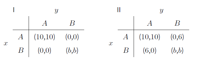 |
Table 2 shows the two classes of coordination games that are analysed. The parameter \(b\) is set to an element of \(\{2,4,6,8,10\}\). Hence, (A; A) and (B; B) are always pure Nash equilibria, and the classes cover games with different relationships between the two equilibria. In game I, the outcome (A; A) is efficient and risk-dominant as long as b < 10. If b = 10, both outcomes (A; A) and (B; B) are efficient, and there is no risk-dominance relationship between them. In game II, the outcome (A; A) is efficient as well. But it is risk-dominant only if b > 4. In case of b = 4, there is no risk-dominance relationship, and, if b > 4, (B; B) risk-dominates (A; A) although it may be inefficient (b < 10).
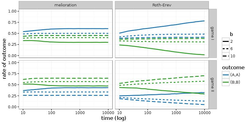
If these games are repeatedly played by the same two persons, melioration learning as well as Roth-Erev predict a pure Nash equilibrium. In Figure 2, results of simulations with 50.000 pairs of actors are shown (\(\varepsilon = 0.1\)). Distributions over the four outcomes of the games are measured at the 1.000th round of the simulation. While melioration learning has stabilised at this round, Roth-Erev continuous to evolve (see Figure 9 in the appendix). Nevertheless, most pairs have already coordinated their choices to (A; A) or (B; B). The latter outcome is observed even if it is inefficient and risk-dominated (game I with b < 10).
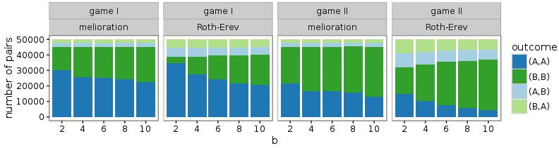
More specifically, the frequency of (B; B) increases with b and is higher in game II than game I. The first effect is due to the larger rewards for choosing alternative B. The second effect occurs because, in both learning models, the attachment of values (\(V_t(\cdot)\) or \(P_t(\cdot)\)) to the alternatives takes place irrespectively of the choice of the other actor. Since \(\varepsilon > 0\), also the outcomes (A; B) and (B; A) emerge occasionally. This implies that the value of action B is slightly higher in game II.
The following simulations were run with groups of 50 actors, each of whom interacted with multiple partners. A network specified the structure of interactions. While the vertices of the network represent the actors, an edge exists between two vertices if the corresponding actors repeatedly take part in the same coordination game. The actors do not distinguish between the partners. Only one set of values is maintained, and the partner is not taken into consideration when choosing between the alternatives. This means that, given the games of Table 2, all members of a connected component of the network should agree on a single alternative in order to avoid the inferior outcomes (A; B) and (B; A).
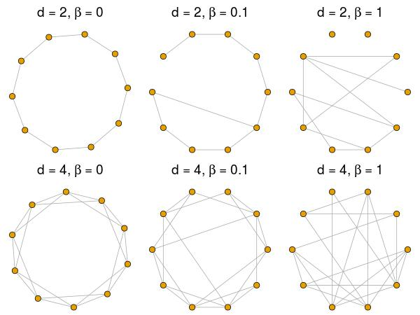
In particular, the small-world (\(\beta\)-)model of Watts (1999, p. 67) is used to specify the structure of interactions. This model has two parameters: the average number of neighbours \(d \in \{2,4,6,\dots\}\) and the probability of rewiring \(\beta \in [0,1]\). While the small-world model reproduces only some properties that are found in real networks, it covers two important ones: high clustering and low distances. If \(\beta = 0\), clustering and distance are maximal. The network resembles a one-dimensional lattice in which each actor has exactly d neighbours (see Figure 3). With an increasing \(\beta\), more and more edges are rewired from a close neighbour to a random actor of the network. In case of \(\beta=1\), the average distance is minimal and no clustering remains. Networks with high levels of clustering but still low distances are found for small but strictly positive values of \(\beta\).
The small-world model is an excellent technique to study the effects of restrictive network structures. If \(\beta=0\), interactions are limited to rigid clusters. In large networks, this hinders the establishment of a convention because a high number of rounds is required to coordinate the actions between distant parts of the network. If (\beta\) increases, interactions take place also with distant regions. This may accelerate the agreement on a convention.
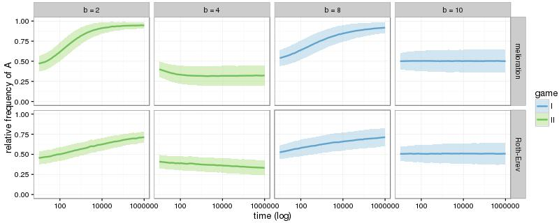
Each of the following plots reports the outcomes of 1.000 groups of 50 actors. First, one-dimensional lattices with \(d = 2\) are analysed. This means that the networks resemble polygons. The plots of Figure 4 show the relative frequencies of alternative A over the first 1.000 rounds of the simulations. The frequencies are averaged over all groups by reporting the mean and standard deviation (ribbon in plots).
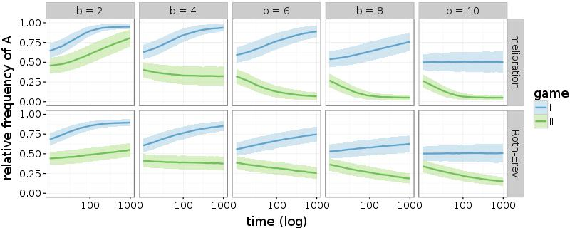
In case of melioration learning, groups that play game I with b < 8 or game II with b > 4 are able to coordinate their decisions within the first 1.000 rounds. With further rounds of the simulations, all groups eventually establish a convention as long as there is a risk-dominant equilibrium (game I with \(b \neq 10\) and game II with \(b \neq 4\)). This is shown in the appendix (Figure 10). The results of the simulations with Roth-Erev seem similar, but the convergence takes place substantially more slowly. Nevertheless, the simulations confirm the result of Young (1998, p. 98): the groups establish a convention by coordinating their members’ choices to a risk-dominant equilibrium. This holds true even if the risk-dominant equilibrium is inefficient (game II with 4 < b < 10).
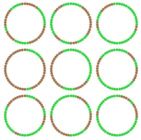
In situations without risk-dominant equilibrium, both alternatives persists. Figure 5 shows nine of the 1.000 groups that played game I with b = 10. Different colours indicate different choices at the 1.000th round of the simulations (without exploration). The actors are partitioned into clusters, which are stable over time. Actors on the edge of a cluster have no incentive to change behaviour, for they receive a reward of ten from one of the partners and zero reward from the other one. Switching to the other alternative would not change this pattern, unless exactly one of the two partners switches as well.
The difficulty of establishing a convention in games without risk-dominant outcome can be traced back to the restrictive structure of polygons (small-world networks with d = 2 and \(\beta\) = 0). First, the convergence to a single alternative is made possible by adding more connections to the network. Figure 6 shows this effect for the melioration learning model and game I with b = 10. The relative frequencies of alternative A are measured at the 1.000th round of the simulations and for each of the 1.000 groups separately. The histograms picture the frequencies of groups with a particular relative frequency. The plots indicated that a higher number of network partners d enables a larger fraction of groups to choose a single alternative. If d = 20, approximately half of the groups can already coordinate their choices within 1.000 rounds. All groups achieve a convention in complete or nearly complete networks (d = 40 or d = 50). While in half of the groups, everyone chooses A, in the other half, a convention of selecting alternative B emerges.
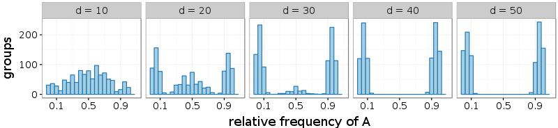
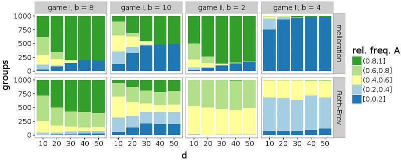
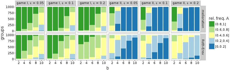
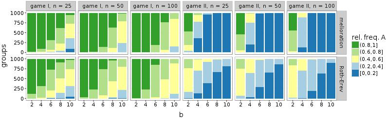
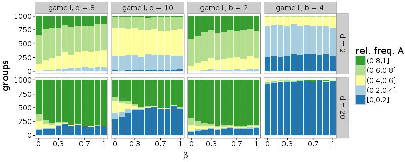
Figure 7 shows similar histograms for all problematic situations: game I with \(b \in \{8,10\}\) and game II with \(b \in \{2,4\}\). To make the plots accessible, the histograms are reduced to five intervals: [0; 0:2], (0:2; 0:4], (0:4; 0:6], (0:6; 0:8], and (0:8; 1]. In case of melioration learning, the frequencies of the two outer intervals increase with d, which means that more and more groups agree upon a common alternative. Since the relative frequencies are measured at the 1.000th round of the simulations, a comparison with Figure 4 reveals that a high number of interaction partners (given by d) either accelerates the establishment of conventions (game I with b = 8 and game II with b = 2) or makes it possible in the first place (game I with b = 10 and game II with b = 4). In simulations of the Roth-Erev model, the number of contacts d increases the frequency of conventions only in game I and at a slower rate. In game II, Roth-Erev is incapable of quickly coordinating a group.
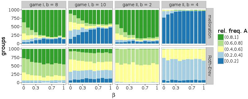
Furthermore, also a high probability of rewiring (\(\beta\)) facilitates the common choice of a single alternative. Similar to a larger number of partners, connections to random agents support the coordination within the network. Figure 8 illustrates this effect for networks with d = 10. While simulations of melioration learning indicate that the frequencies of the inner intervals, which contain groups without convention, decrease with \(\beta\), this parameter affects the results only slightly in case of Roth-Erev.
In summary, a more dense or a more random structure supports the establishment of a convention. In game I with b = 8 and game II with b = 2, a convergence to the risk-dominant outcome (A; A) is seen. In the games without risk-dominance relation, the results differ. While the groups are equally divided among the two efficient outcomes in game I with b = 10, the actors settle on the inefficient outcome (B; B) in game II with b = 4.
Conclusion
With melioration learning, a simple and empirically grounded model of reinforcement learning was shown to explain the emergence of conventions. In contrast to previous research on this subject (e.g. Young 1998; Berninghaus & Schwalbe 1996; Buskens & Snijders 2016), this study proves that conventions emerge even if the actors are neither aware of the payoff structure nor the decisions of other actors. However, melioration learning should not be seen as more general than the previous models. It applies to different settings. Since humans can be assumed to take various information into account, the previous models might be more appropriate in situations in which information on payoffs and other actors is available. For other settings, melioration learning should be used.
In some aspects, melioration learning is actually similar to the behavioural model of Young (1998). The actors are myopic, take past occurrences into account, and make random mistakes. However, unlike the earlier model, less strict assumptions about available information and the actors’ cognitive skills are required. Although they must be able to observe their payoffs and to aggregate them to average values, no advanced reasoning about the given situation is necessary. Moreover, apart from the exploration rate, an alternative with the highest average value is selected with certainty. No further assumptions about probabilities of choice or stochastically independent decisions (cf. Roth-Erev) are needed.
The computer simulations revealed that the outcomes of melioration are largely in line with the results of Young (1998). In the long run, a convention is established by converging to a risk-dominant Nash equilibrium of the stage game. Given the particular settings of the simulations, the final outcome is independent of the network structure. However, the network structure is relevant in two other respects. First, it affects the speed of convergence in games with risk-dominant Nash equilibrium. Second, it impedes or enables the establishment of conventions in games without risk-dominance relationship.
While games without risk-dominance relationship have not been considered by Young (1998), Buskens & Snijders (2016, p. 8) stated that, in these situations (corresponding to RISK = 0.5), "there are no effects of network characteristics whatsoever". For example, in game II with b = 4, the model of Buskens & Snijders (2015) predicts “an average percentage of actors playing [B] of 50% at the end of the simulation runs”. However, in the simulations with melioration learning, this percentage depends on the network structure, and may be close to 100% if the randomness parameter \(\beta\) or the average number of partners \(d\) is high (Figures 7 and 8). Hence, the effects of network structure differ between the model of Buskens & Snijders (2016) and melioration learning.
In two-person games, even the risk-dominated Nash equilibrium emerges with high frequency. Only if interactions take place with multiple partners and in large groups, the risk-dominant outcome prevails. The same effect was seen in simulations with the Roth-Erev model. Generally, the results of melioration and Roth-Erev correspond to each other. However, Roth-Erev converges considerably more slowly than melioration learning to a stable state with convention. Furthermore, the effect of network structures is less pronounced and partly missing in simulations with Roth-Erev.
Currently, there are no empirical confirmations of the predictions of the simulations. On the contrary, experimental studies yielded a likely convergence to the efficient (payoff-dominant) outcome, even if it is risk-dominated (e.g. Frey et al. 2012). Additionally, network effects on the outcome have been observed (Berninghaus et al. 2002; Cassar 2007). In these experiments, the subjects knew the payoff structure of the game, and information about the decisions of other actors was available. Therefore, melioration learning is inadequate in situations in which this kind of information is provided. However, in other situations, melioration learning might be a valid model of individual behaviour. Empirical studies that corroborate this hypothesis are still missing.
Acknowledgements
This article is based on material that has formed part of my doctoral thesis, which is available at http://nbn-resolving.de/urn:nbn:de:bsz:15-qucosa-216771. Advice given by Thomas Voss has been of great help in the development of this work. Three anonymous reviewers have helped to significantly improve the manuscript. Furthermore, I acknowledge support from the German Research Foundation (DFG) and Leipzig University within the program of Open Access Publishing,Notes
- A connected component is a part of a network in which every member is reachable by every other member via a sequence of edges.
Appendix A: Further results and sensitivity analysis
Figure 9 presents the temporal development of decisions in two-person coordination games. While melioration stabilises after approximately 100 interactions, Roth-Erev takes more than 10.000 interactions in some settings.
Similarly, the Roth-Erev model converges more slowly in n-way coordination games. Figure 10 depicts data from the same simulations as Figure 4 but for longer time periods. Only the difficult cases are shown. Melioration learning stabilises at the risk-dominant equilibria if one exists. The actors with Roth-Erev develop in the same direction but even 1.000.000 interactions do not suffice to converge under the present conditions.
The simulations of Figure 4 (\(d\) = 2 and \(\beta\)= 0) were repeated for different exploration rates \(\varepsilon\). The relationship between parameter \(b\) of the game and the distribution of groups is robust against small changes in \(\varepsilon\) (Figure 11). A group’s ability to coordinate its members’ choices still depends on the reward \(b\). Only in case of Roth-Erev and game II, the establishment of a convention is further impeded by high levels of exploration (\(\varepsilon\) = 0.2).
Finally, the effect of the rewiring parameter \(\beta\) was tested for robustness by altering the second parameter \(d\). In Figure 13, only results from simulations with melioration learning are included. On the one hand, the establishment of a convention is not facilitated by \(\beta\) if \(d\) = 2. In case of small \(d\) and \(\beta\) > 0, a network is often disconnected, which hinders the coordination. On the other hand, the relationship between the randomness parameter \(\beta\) and the distribution of choices is stronger in networks with a high average number of partners (\(d\) = 20). This corresponds to the result that a large number of connections or a high level of randomness supports the establishment of a convention.
Appendix B: Simulation software
The simulations were run on NetLogo (Wilensky 1999) with two extensions that must be manually installed. The extensions are available at
https://github.com/JZschache/NetLogo-ql
andhttps://github.com/JZschache/NetLogo-games
The NetLogo-file of the simulations can be found athttps://github.com/JZschache/NetLogo-games/blob/master/models/n-way-games.nlogo
The next section deals with the installation of both extensions. Afterwards, the usage and architecture of the ql-extension is comprehensively described. It is the core of the simulations, for it implements melioration learning and handles the parallelisation of the simulations. In the last section, a short introduction to the games-extension is given. It facilitates the definition of two-person games in NetLogo.
Installation
First, install NetLogo (tested with NetLogo 5.2.1). Second, create a directory named ql in the extensions subdirectory of the NetLogo installation (see also http://ccl.northwestern.edu/netlogo/docs/extensions.html). Third, download all files from the repository and move them to the newly created directory. For example:
git clone https://github.com/JZschache/NetLogo-ql.gitmvNetLogo-ql/extensions/qlpath-to-netlogo/extensions
Similarly, the games-extension is installed by creating a directory named games in the extensions subdirectory of the NetLogo program, downloading all files, and moving them to the newly created directory:
git clone https://github.com/JZschache/NetLogo-games.git

mv NetLogo-games/extensions/games path-to-netlogo/extensions
Since the games-extension is used in combination with the ql-extension, the configuration file extensions/ql/application.conf must be edited:
enable-parallel-mode is set to true.
The ql-extension
The ql-extension enables a parallelised simulation of agents who make decisions by melioration learning. In order to explain the usage of this extension, listing 1 contains some parts of n-way-games.nlogo.
Listing 1: Some parts of n-way-games.nlogo
After the turtles are created, the ql-extension is initialised by ql:init. If the variables exploration-rate and exploration-method are specified before ql:init is called, these values are used for the agents (otherwise, default values are employed; see: application.conf).
The exploration rate is a positive number. Note that this rate cannot be interactively changed during the simulation (as it is usually possible in NetLogo). The method of exploration “epsilon-greedy” denotes the implementation of algorithm 1. Another possible value is “Roth-Erev”.
As stated in the main text, the melioration algorithm requires the agents to use and modify values (\(V\)) when making decisions. The current state of these values are accessed via the agent variable q-values, which is a list of numbers. This list is automatically updated during the simulation if defined by turtles-own. Besides the values, also the frequencies of choice (frequencies) are continuously updated. The names of the variables can be changed in the configuration file (application.conf).
Similar to the “small worlds” model that is available from the NetLogo commons (http://ccl.northwestern.edu/netlogo/models/SmallWorlds), the procedure of listing 1 embeds the turtles in a one-dimension lattice with \(d\) = 2. It builds a set of groups, which is named group-structure. Each group contains two agents (neighbours of the network) and is created by a special reporter: ql:create-group. This reporter creates a group from a list of pairs. Each pair specifies an agent and a list of integers that stand for the choice alternatives. In the previous simulations, the choice alternatives were the actions A and B of the coordination game.
After turtles and network have been set up in the NetLogo world, the process logic of the simulation must be implemented. However, the ql-extension alters the usual way of working with NetLogo because it parallelises the calculations. In contrast to most NetLogo models, the simulations are controlled by the ql-extension, and NetLogo is used as a convenient platform to specify the situation. This is explained in the following.
Simulations with the ql-extension are started and stopped by ql:start and ql:stop. After starting the simulation, three functions are called repeatedly by the ql-extension and, hence, must be implemented in the NetLogo model. By default, the functions are named get-groups, get-rewards and update (the names can be changed in the file application.conf). The first function is used by the extension to retrieve a set of groups in which the interaction takes place. In the example of the previous simulations, these are two-person groups of network neighbours. The second function is responsible for calculating the rewards of a group of agents (specified by the coordination game). It comes with exactly one parameter (headless-id). The third function is executed repeatedly after every agent has received a reward. In listing 2, examples for all three functions are given.
Listing 2: Sample NetLogo code of the three functions
The ql-extension is able to parallelise the simulation and utilise multiple cores by deploying the Akka framework (Akka 2.0.5, http://akka.io). Akka handles the difficulties of data sharing and synchronisation by a message-passing architecture. More concretely, it requires the implementation of “Akka actors” that run independently and share data by sending messages to each other.
Simulations are parallelised in two ways. First, the NetLogo threads are not used for the ql-extension, which means that the latter runs independently of the former. Second, the learning and decision-making of agents take place simultaneously because the ql-extension runs on multiple threads.
Nevertheless, many parts of the simulation are executed by NetLogo, which does not parallelise naturally. This is a major bottleneck of the simulations. The ql-extension must wait for NetLogo to finish its calculations. The ql-extension solves this problem by the operation of multiple concurrently running instances of NetLogo. This feature is enabled by setting enable-parallel-mode to true (application.conf).
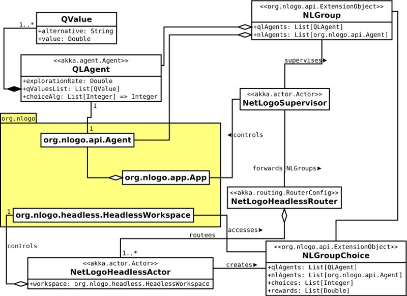
For a better understanding of the parallel mode, the architecture of the ql-extension is illustrated by the class diagram of Figure 14. It clarifies the connection between the extension and the NetLogo package org.nlogo. It also shows how concurrency is implemented by “Akka actors”. First, each NetLogo agent (a turtle or a patch) is linked to an “Akka actor”. This is realised by the QLAgent class, which constitutes the counterpart of a NetLogo agent in the ql-extension. It is characterised by an exploration rate, a list of QValues, and a decision-making algorithm (e.g. “epsilon-greedy”). A QValue instance is created for each alternative and specifies its current value. The decision-making algorithm returns an element of a list of alternatives (a list of integers). It uses the exploration rate and the QValues.
Agents are grouped together by the class NLGroup. This is a subclass of org.nlogo.api.ExtensionObject, which makes it accessible within NetLogo code. It consists of NetLogo agents and the corresponding QLAgents. Objects of this class are created by the command ql:create-group.
The main “Akka actor” of the extension is the NetLogoSupervisor. There is only one instance of this class. The NetLogoSupervisor has mutliple tasks. For example, it supervises all NLGroups and continuously triggers the choices of agents. The speed of the repeated trigger is regulated by the corresponding slider of the NetLogo interface. When triggering the choice of agents, a list of NLGroups is forwarded to the NetLogoHeadless-Router. Depending on the number of NetLogoHeadlessActors, the router splits this list into multiple parts. Afterwards, the NetLogoHeadlessActors handle the choices of the agents, and the NetLogoSupervisor is free to do other things.
When initialising the NetLogoSupervisor by ql:init, several headless workspaces of NetLogo are started in the background. Headless means that no graphical user interface is deployed. The number of headless workspaces is specified in the configuration file (application.conf). A separate NetLogoHeadlessActor controls each headless NetLogo instance. This actor continuously receives a list of NLGroups.
The headless NetLogo workspaces and the NetLogoHeadlessActors were added to the ql-extension in order to improve the performance. Their only task is to repeatedly calculate the rewards of a group of agents. The performance of repeatedly calling a function is optimised by compiling this function only once. This is problematic because the NetLogo extensions API does currently not support the passing of arguments to a com-piled function (see https://github.com/NetLogo/NetLogo/issues/413). A solution was mentioned by Seth Tisue in the corresponding discussion (https://groups.google.com/forum/#!msg/netlogo-devel/8oDmCRERDlQ/0IDZm015eNwJ) and is implemented in the ql-extension. This solution requires that each NetLogoHeadlessActor is identified by a unique number. This number is forwarded to the reward function when it is called by the NetLogoHeadlessActor. The reward function calls ql:get-group-list with the identifying number and receives a list of NLGroupChoices. Besides the agents, an NLGroupChoice also contains a list of agents’ decisions. The agents and their choices are accessed by the reporters ql:get-agents and ql:get-decisions. The rewards are set to an NLGroupChoice by ql:set-rewards. The reward function can also be used to update the (NetLogo) agents directly, e.g. by moving the agents within the NetLogo world or by setting variables. Since the agents are passed from the main NetLogo instance, the changes take effect in this instance as well. Finally, the reward function must return a new list of NLGroupChoices that correspond to the received list but with the rewards set.
The following list summarises the usage of the main commands of the ql-extension:
ql:initinitialises the ql-extension by specifying a turtleset or a patchset.ql:create-groupcreates a group from a list of pairs. Each pair is a list of two elements: first, an agent and, second, a list of integers (the alternatives). An object of typeNLGroupis returned.ql:set-group-structuretakes a list of objects of typeNLGroupas parameter. It sets a static group structure.ql:startorql:stopstarts or stops the simulation.ql:get-group-listcan only be called from the reward function and must forward theheadless-id. It returns a list of objects of typeNLGroupChoice.ql:get-agentsreturns the list of NetLogo agents (turtles or patches) that are held by anNLGroupChoice.ql:get-decisionsreturns the list of decisions that are held by anNLGroupChoice. The indices of the decisions correspond to the indices of the agents that are held by theNLGroupChoicesuch that the decision at index i belongs to the agent at index i.ql:set-rewardssets a list of rewards for the decisions that are held by anNLGroupChoice. It returns a copy of theNLGroupChoicewith the rewards attribute set. The indices of the rewards must correspond to the indices of the agents that are held by theNLGroupChoicesuch that the reward at index i belongs to the agent at index i.
The games-extension
The games-extension provides a convenient way to define normal-form game-theoretic situations. Optimal points and Nash equilibria are calculated and returned to NetLogo in a well-arranged form. A two-person game can be defined manually or by a predefined name. The first way is demonstrated with the help of Figure 15.
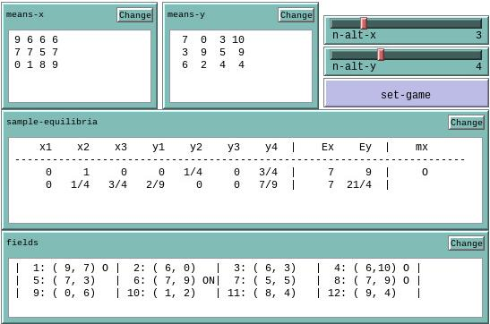
In Figure 15, two NetLogo input fields named means-x and means-y are seen. Each field contains the mean rewards of player x or player y, respectively, given the choices of both players. Player x is the row-player in both fields. In order to create a game from the two input fields, two game-matrices must be created by the reporter games:matrix-from-row-list and joint together by games:two-persons-game (see function set-game in n-way-games.nlogo).
The second way of creating a two-person game requires only a name and, occasionally, the numbers of alter-natives for both players:
The reporter games:two-persons-gamut-game is based on the Gamut library (http://gamut.stanford.edu). Gamut makes available over thirty games that are commonly found in the economic literature. The games-extension currently supports the following parameters as name of a game:
- "BattleOfThSexes" "Chicken"
- "CollaborationGame"
- "CoordinationGame"
- "DispersionGame" (considers first number of alternatives)
- "GrabTheDollar" (considers first number of alternatives)
- "GuessTwoThirdsAve" (considers first number of alternatives)
- "HawkAndDove"
- "MajorityVoting" (considers first number of alternatives)
- "MatchingPennies"
- "PrisonersDilemma"
- "RandomGame" (considers both numbers of alternatives)
- "RandomZeroSum" (considers both numbers of alternatives)
- "RockPaperScissors"
- "ShapleysGame"
Further commands of the games-extension are described in the following list:
games:game-matrixreturns a game-matrix of a game.games:matrix-as-pretty-stringsconverts a game-matrix into a list of lists of strings. The strings are “pretty” because it is accounted for differences in length of the numbers by inserting spaces. An additional general cell shift can be specified by a second parameter, for example two spaces (" ").games:matrix-transposetakes a game-matrix as parameter and returns the transpose of this matrix. This reporter assists when defining symmetric games. The input matrix must be quadratic.games:get-rewardreturns an entry of a game-matrix. Therefore, three parameters are required: the matrix, a row index, and a column index.games:get-solutions-stringcan be used to update a NetLogo input field (see sample-equilibria in Figure 15). It prints (strictly) mixed Nash equilibria (if some are found). It also prints the expected reward of each player and indicates, by anOin the last column, whether a solution is (Pareto) optimal compared to the other (pure and mixed) solutions. A second parameter is used to adjust the cell shift.games:get-fields-stringcan be used to update a NetLogo input field (see fields in Figure 15). It prints a joint payoff matrix. Each field of the matrix contains an index and the mean rewards as specified by the game. It also indicates the pure Nash equilibria (N) and pure (Pareto) optima (O). A second parameter is used to adjust the cell shift.games:pure-solutionsreturns a list of boolean values, one for each field of the joint payoff matrix (as given bygames:get-fields-string). Each value indicates whether this field is a pure Nash equilibrium.games:pure-optimareturns a list of boolean values, one for each field of the joint payo matrix (as given bygames:get-fields-string). The boolean value indicates whether this field is (Pareto) optimal com-pared to the other (pure and mixed) solutions.
While pure Nash equilibria are easily identified, the search for a Nash equilibrium in general is computationally intensive (see e.g. Shoham & Leyton-Brown 2009, ch. 4). Nevertheless, existing algorithms run e iciently in practice (e.g. Codenotti et al. 2008). One of the better known (but not the fastest) one (Shoham & Leyton-Brown 2009, p. 91) is the Lemke-Howard algorithm (Lemke & Howson 1964). This algorithm is implemented in the games-extension (as given by Codenotti et al. 2008). Even though the Lemke-Howard algorithm necessarily finds a Nash equilibrium, it is generally not able to find all equilibria (Shoham & Leyton-Brown 2009, p. 98). The implementation of the games-extension tries to find multiple equilibria by starting the algorithm with every possible variable that can be part of the solution (see the pseudocode in Shoham & Leyton-Brown 2009, p. 96). This step is repeated for every solution that has already been calculated. Since not all Nash equilibria are found, the input field of the NetLogo interface was named sample-equilibria.
Furthermore, the problem of stating whether a Nash equilibrium is Pareto optimal is NP-hard (Shoham & Leyton-Brown 2009, p. 102). With a finite set of outcomes, the search for the optimal ones can be completed in polynomial time (and, on average, even in linear time, Godfrey et al. 2007). Consequently, the games-extension inspects only the pure and mixed Nash equilibria that are found directly or by the Lemke-Howard algorithm. The labelling of an outcome by an O must, hence, be understood relatively to the outcomes that are shown.
References
ANTONIDES, G. & Maital, S. (2002). Effects of feedback and educational training on maximization in choice tasks: Experimental-game evidence. The Journal of Socio-Economics, 31(2), 155–165. [doi:10.1016/S1053-5357(01)00130-5]
BABICHENKO, Y. (2012). Completely uncoupled dynamics and Nash equilibria. Games and Economic Behavior, 76(1), 1–14.
BANISCH, S. (2016). Markov Chain Aggregation for Agent-Based Models. Springer International Publishing. [doi:10.1007/978-3-319-24877-6]
BARTO, A. G., Sutton, R. S. & Watkins, C. J. C. H. (1990). ‘Learning and sequential decision making’. In M. Gabriel & J. Moore (Eds.), Learning and Computational Neuroscience: Foundations of Adaptive Networks, (pp. 539–602). Cambridge, MA: MIT Press.
BAUM, W. M. (1979). Matching, undermatching, and overmatching in studies of choice. Journal of the Experimental Analysis of Behavior, 32(2), 269–281. [doi:10.1901/jeab.1979.32-269]
BELLMAN, R. E. (1957). A Markov decision process. Journal of Mathematics and Mechanics, 6(5), 679–684.
BENDOR, J., Diermeier, D. & Ting, M. (2007). Comment: Adaptive models in sociology and the problem of empirical content. American Journal of Sociology, 112(5), 1534–1545. [doi:10.1086/512962]
BERNINGHAUS, S. K., Ehrhart, K.-M. & Keser, C. (2002). Conventions and local interaction structures: Experimental evidence. Games and Economic Behavior, 39(2), 177–205.
BERNINGHAUS, S. K. & Schwalbe, U. (1996). Conventions, local interaction, and automata networks. Journal of Evolutionary Economics, 6(3), 297–312. [doi:10.1007/BF01193635]
BORRERO, J. C., Crisolo, S. S., Tu, Q., Rieland, W. A., Ross, N. A., Francisco, M. T. & Yamamoto, K. Y. (2007). An application of the matching law to social dynamics. Journal of Applied Behavior Analysis, 40(4), 589–601.
BRENNER, T. (2006). ‘Agent learning representation: Advice on modelling economic learning’. In L. Tesfatsion & K. L. Judd (Eds.), Handbook of Computational Economics. Agent-based Computational Economics, vol. 2. North-Holland. [doi:10.1016/s1574-0021(05)02018-6]
BRENNER, T. & Witt, U. (2003). Melioration learning in games with constant and frequency-dependent payoffs. Journal of Economic Behavior & Organization, 50(4), 429–448.
BUSH, R. R. & Mosteller, F. (1964). Stochastic Models for Learning. New York: Wiley, 2nd edn.
BUSKENS, V. & Snijders, C. (2016). Effects of network characteristics on reaching the payoff-dominant equilibrium in coordination games: A simulation study. Dynamic Games and Applications, 6(4), pp 477–494.
CAMERER, C. F. (2003). Behavioral Game Theory: Experiments in Strategic Interaction. Princeton, NJ: Princeton University Press.
CASSAR, A. (2007). Coordination cooperation in local, random and small world networks: Experimental evidence. Games and Economic Behavior, 58(2), 209–230.
CLAUS, C. & Boutilier, C. (1998). The dynamics of reinforcement learning in cooperative multiagent systems. In AAAI ’98 Proceedings of the Fifteenth National Conference on Artificial Intelligence, (pp. 746–752).
CODENOTTI, B., Rossi, S. D. & Pagan, M. (2008). An experimental analysis of Lemke-Howson algorithm. https://arxiv.org/abs/0811.3247.
FOSTER, D. P. & Young, H. P. (2006). Regret testing: Learning to play Nash equilibrium without knowing you have an opponent. Theoretical Economics, 1(3), 341–367.
FREY, V., Corten, R. & Buskens, V. (2012). Equilibrium selection in network coordination games: An experimental study. Review of Network Economics, 11(3).
GERMANO, F. & Lugosi, G. (2007). Global Nash convergence of Foster and Young’s regret testing. Games and Economic Behavior, 60(1), 135–154. [doi:10.1016/j.geb.2006.06.001]
GODFREY, P., Shipley, R. & Gryz, J. (2007). Algorithms and analyses for maximal vector computation. The VLDB Journal, 16, 5–28.
GOMES, E. R. & Kowalczyk, R. (2009). ‘Dynamic analysis of multiagent Q-learning with \(\varepsilon\)-greedy exploration’. In A. P. Danyluk, L. Bottou & M. L. Littman (Eds.), Proceedings of the 26th Annual International Conference on Machine Learning, ICML 2009, Montréal, Canada, (pp. 369–376). ACM.
HARSANYI, J. C. & Selten, R. (1992). A general theory of equilibrium selection in games. Cambridge, MA: The MIT Press, 2nd edn.
HERRNSTEIN, R. J. (1997). The Matching Law. Papers in Psychology and Economics. Cambridge, Mass. & London, England: Harvard University Press.
HERRNSTEIN, R. J., Loewenstein, G. F., Prelec, D. & Vaughan, W. (1993). Utility maximization and melioration: Internalities in individual choice. Journal of Behavioral Decision Making, 6(3), 149–185.
HERRNSTEIN, R. J. & Vaughan, W. (1980). ‘Melioration and behavioral allocation’. In J. E. R. Staddon (Ed.), Limits to Action: The Allocation of Individual Behaviour, chap. 5, (pp. 143–175). New York: Academic Press. [doi:10.1016/B978-0-12-662650-6.50011-8]
IZQUIERDO, L. R. & Izquierdo, S. S. (2012). ‘Reinforcement learning’. In N. M. Seel (Ed.), Encyclopedia of the Sciences of Learning, (pp. 2796–2799). Springer US.
IZQUIERDO, L. R., Izquierdo, S. S., Galán, J. M. & Santos, J. I. (2009). Techniques to understand computer simulations: Markov chain analysis. Journal of Artificial Societies and Social Simulation, 12(1), 6: https://www.jasss.org/12/1/6.html.
IZQUIERDO, L. R., Izquierdo, S. S., Gotts, N. M. & Polhill, J. G. (2007). Transient and asymptotic dynamics of reinforcement learning in games. Games and Economic Behavior, 61(2), 259–276.
JAAKKOLA, T., Jordan, M. I. & Singh, S. P. (1994). On the convergence of stochastic iterative dynamic programming algorithms. Neural Computation, 6(6), 1185–1201. [doi:10.1162/neco.1994.6.6.1185]
KANDORI, M., Mailath, G. J. & Rob, R. (1993). Learning, mutation, and long run equilibria in games. Econometrica, 61(1), 29–56.
LEMKE, C. E. & Howson, J. T. (1964). Equilibrium points of bimatrix games. Journal of the Society for Industrial and Applied Mathematics, 12(2), 413–423. [doi:10.1137/0112033]
LOEWENSTEIN, Y. (2010). Synaptic theory of replicator-like melioration. Frontiers in Computational Neuroscience, 4, 17.
MACY, M. W. (1991). Learning to cooperate: Stochastic and tacit collusion in social exchange. American Journal of Sociology, 97(3), 808–843. [doi:10.1086/229821]
MACY, M. W. & Flache, A. (2002). Learning dynamics in social dilemmas. Proceedings of the National Academy of Sciences, 99(Suppl 3), 7229.
MAZUR, J. E. (1981). Optimization theory fails to predict performance of pigeons in a two-response situation. Science, 214(4522), 823–825. [doi:10.1126/science.7292017]
MCDOWELL, J. J. (1988). Matching theory in natural human environments. The Behavior Analyst, 11(2), 95–109.
NETH, H., Sims, C. R. & Gray, W. D. (2005). Melioration despite more information: The role of feedback frequency in stable suboptimal performance. In Proceedings of the Human Factors and Ergonomics Society 49th Annual Meeting, (pp. 357–361). [doi:10.1177/154193120504900330]
NOWÉ, A., Vrancx, P. & Hauwere, Y.-M. D. (2012). ‘Game theory and multi-agent reinforcement learning’. In M. Wier-ing & M. van Otterlo (Eds.), Reinforcement Learning. State-of-the-Art, (pp. 441–470). Berlin and Heidelberg: Springer.
Pierce, W. D. & Epling, W. F. (1983). Choice, matching, and human behavior. A review of the literature. The Behavior Analyst, 6(1), 57–76.
PRADELSKI, B. S. & Young, H. P. (2012). Learning efficient Nash equilibria in distributed systems. Games and Economic Behavior, 75(2), 882–897.
ROTH, A. E. & Erev, I. (1995). Learning in extensive-form games: Experimental data and simple dynamic models in the intermediate term. Games and Economic Behaviour, 8(1), 164–212. [doi:10.1016/S0899-8256(05)80020-X]
SAKAI, Y., Okamoto, H. & Fukai, T. (2006). Computational algorithms and neuronal network models underlying decision processes. Neural Networks, 19(8), 1091 – 1105
SANDHOLM, T. W. & Crites, R. H. (1995). On multiagent Q-learning in a semi-competitive domain. In G. Weiß & S. Sen (Eds.), Adaptation and Learning in Multiagent Systems, IJCAI’95 Workshop, Montréal, Canada, August 1995, Proceedings, Lecture Notes in Artificial Intelligence 1042, (pp. 191–205). Springer.
SCHELLING, T. C. (1960). The strategy of conflict. Cambridge: Harvard University Press.
SHOHAM, Y. & Leyton-Brown, K. (2009). Multiagent Systems. Algorithmic, Game-Theoretic, and Logical Foundations. New York: Cambridge University Press.
SHTEINGART, H. & Loewenstein, Y. (2014). Reinforcement learning and human behavior. Current Opinion in Neurobiology, 25, 93–98.
STADDON, J. E. R. (2001). Adaptive Dynamics. The Theoretical Analysis of Behavior. Cambridge, Mass. & London, England: The MIT Press.
STADDON, J. E. R. & Cerutti, D. T. (2003). Operant conditioning. Annual Review of Psychology, 54(1), 115–144.
SUTTON, R. S. & Barto, A. G. (1998). Reinforcement learning. An Introduction. Cambridge, Massachusetts, and London, England: The MIT Press.
THORNDIKE, E. L. (1932). The Fundamentals of Learning. New York: Teachers College, Columbia University.
TUNNEY, R. J. & Shanks, D. R. (2002). A re-examination of melioration and rational-choice. Journal of Behavioral Decision Making, 15(4), 291–311. [doi:10.1002/bdm.415]
VAUGHAN, W. (1981). Melioration, matching, and maximization. Journal of the Experimental Analysis of Behavior, 36(2), 141–149.
VAUGHAN, W. & Herrnstein, R. J. (1987). ‘Stability, melioration, and natural selection’. In L. Green & J. H. Kagel (Eds.), Advances in Behavioral Economics, vol. 1, (pp. 185–215). Norwood, NJ: Ablex.
VOLLMER, T. R. & Bourret, J. (2000). An application of the matching law to evaluate the allocation of two- and three-point shots by college basketball players. Journal of Applied Behavior Analysis, 33(2), 137–150.
WATKINS, C. J. C. H. (1989). Learning from delayed rewards. Ph. D. thesis, University of Cambridge, England-Vaughan.
WATKINS, C. J. C. H. & Dayan, P. (1992). Q-learning. Machine Learning, 8(3-4), 279–292.
WATTS, D. J. (1999). Small worlds: The dynamics of networks between order and randomness. Princeton and Oxford: Princeton University Press.
WILENSKY, U. (1999). Netlogo. http://ccl.northwestern.edu/netlogo/. Center for Connected Learning and Computer-Based Modeling, Northwestern University. Evanston, IL.
WUNDER, M., Littman, M. & Babes, M. (2010). Classes of multiagent Q-learning dynamics with -greedy exploration. In Proceedings of the 27th International Conference on Machine Learning, Haifa, Israel, (pp. 1167–1174).
YOUNG, H. P. (1993). The evolution of conventions. Econometrica, 61(1), 57–84.
YOUNG, H. P. (1998). Individual Strategy and Social Structure. Princeton and Oxford: Princeton University Press.
YOUNG, H. P. (2009). Learning by trial and error. Games and Economic Behavior, 65(2), 626–643.