Luis R. Izquierdo, Segismundo S. Izquierdo, José Manuel Galán and José Ignacio Santos (2009)

Techniques to Understand Computer Simulations: Markov Chain Analysis

Journal of Artificial Societies and Social Simulation vol. 12, no. 1 6
<https://www.jasss.org/12/1/6.html>

For information about citing this article, click here

Received: 16-Apr-2008    Accepted: 10-Sep-2008    Published: 31-Jan-2009

Abstract

The aim of this paper is to assist researchers in understanding the dynamics of simulation models that have been implemented and can be run in a computer, i.e. computer models. To do that, we start by explaining (a) that computer models are just input-output functions, (b) that every computer model can be re-implemented in many different formalisms (in particular in most programming languages), leading to alternative representations of the same input-output relation, and (c) that many computer models in the social simulation literature can be usefully represented as time-homogeneous Markov chains. Then we argue that analysing a computer model as a Markov chain can make apparent many features of the model that were not so evident before conducting such analysis. To prove this point, we present the main concepts needed to conduct a formal analysis of any time-homogeneous Markov chain, and we illustrate the usefulness of these concepts by analysing 10 well-known models in the social simulation literature as Markov chains. These models are:

• Schelling's (1971) model of spatial segregation
• Epstein and Axtell's (1996) Sugarscape
• Miller and Page's (2004) standing ovation model
• Arthur's (1989) model of competing technologies
• Axelrod's (1986) metanorms models
• Takahashi's (2000) model of generalized exchange
• Axelrod's (1997) model of dissemination of culture
• Kinnaird's (1946) truels
• Axelrod and Bennett's (1993) model of competing bimodal coalitions
• Joyce et al.'s (2006) model of conditional association

In particular, we explain how to characterise the transient and the asymptotic dynamics of these computer models and, where appropriate, how to assess the stochastic stability of their absorbing states. In all cases, the analysis conducted using the theory of Markov chains has yielded useful insights about the dynamics of the computer model under study.

Keywords:

Computer Modelling, Simulation, Markov, Stochastic Processes, Analysis, Re-Implementation

Supporting material:

Source code used to conduct every experiment and produce every computational figure in this paper

Introduction

1.1

The aim of this paper is to assist researchers in understanding the dynamics of simulation models that have been implemented and can be run in a computer, i.e. computer models. Admittedly, most of what is written here may already be known by many modellers; our hope is that this paper will be useful for newcomers to computer modelling, and for researchers who may not have a strong mathematical background. Specifically, this paper has been written to make and illustrate the following points:

1. A computer model is a deterministic input-output relation, i.e. a function.
2. Any computer model can be re-implemented in many different formalisms (in particular, in any sophisticated enough programming language), leading to alternative representations of the same input-output relation. Thus, we advise researchers to focus on analysing the formal model^[1] that their computer model implements and abstract from the details of the modelling platform where it has been implemented.
3. Pseudorandom number generators give us the potential to simulate random variables within our computer models, and hence use computer models to simulate stochastic processes.
4. Any output obtained from a parameterised model follows a specific probability distribution. This exact probability distribution can be approximated to an arbitrary degree of accuracy by running the model.
5. The formal models that many computer models in the social simulation literature implement can be usefully represented as time-homogeneous Markov chains.
6. Analysing a computer model as a Markov chain can make apparent many features of the model that were not so evident before conducting such analysis.

1.2

The first four points in the list above apply to any computer model and are explained in detail in sections 2, 3, 4 and 5 respectively. They also provide the basic framework for the rest of the paper, which is devoted to explaining and illustrating the usefulness of the theory of Markov chains to analyse computer models. Specifically, sections 6-10 explain what time-homogeneous Markov chains are (section 6) and how to characterise their transient dynamics (section 7), their asymptotic behaviour (sections 8 and 9), and the stochastic stability of their absorbing states (Section 10).

1.3

The theory of Markov chains is a very powerful tool to analyse stochastic systems over time, and is regularly used to model an impressively diverse range of practical systems, such as queuing sequences, re-manufacturing systems, the Internet, inventory systems, reverse logistics, bio-informatics, DNA sequences, genetic networks and data mining (Ching and Ng 2006). However, its use in the social simulation literature is still fairly limited. This paper shows how the theory of Markov chains can be usefully applied in the domain of computational social science. In particular, appendix B includes the analysis of 10 well-known models in the social simulation literature using the concepts explained in this paper. The source code used to conduct every experiment and produce every computational figure in this paper has been included in the supporting material.

Computer models are functions

2.1

A computer model is an implementation —i.e. an explicit representation— of a certain deterministic input-output function in a particular programming language. The word 'function' is useful because it correctly conveys the point that any particular input given to the computer model will lead to one and only one output^[2]. (Obviously, different inputs may lead to the same output.) Admittedly, however, the word 'function' may also mislead the reader into thinking that a computer model is necessarily simple. The computer model may be as complex and sophisticated as the programmer wants it to be but, ultimately, it is just an entity that associates a specific output to any given input, i.e. a function. In any case, to avoid confusion, we will use the term 'formal model' to denote the function that a certain computer model implements. To be sure, the 'formal model' that a particular computer model implements is the abstract entity which is defined by the input-output relation that the computer model executes^[3].

2.2

Thus, running a computer model is just finding out the logical implications of applying a set of unambiguously defined formal rules (which are coded in the program and define the input-output function or formal model) to a set of inputs (Balzer et al. 2001). As an example, one could write the computer program "y = 4·x" and apply it to the input "x = 2" to obtain the output "y = 8". The output (y = 8), which is fully and unequivocally determined by the input (x = 2) and the set of rules coded in the program (y = 4·x), can be seen as a theorem obtained by pure deduction ({x = 2; y = 4·x} ⇒ y = 8). Naturally, there is no reason why the inputs or the outputs should be numbers^[4]; they could equally well be e.g. strings of characters. In the general case, a computer run is a logical theorem that reads: the output obtained from running the computer simulation follows (with logical necessity) from applying to the input the algorithmic rules that define the model. Thus, regardless of its inherent complexity, a computer run constitutes a perfectly valid sufficiency theorem (see e.g. Axtell 2000).

2.3

It is useful to realise that we could always apply the same inference rules ourselves to obtain —by logical deduction— the same output from the given input. While useful as a thought, when it comes to actually doing the job, it is much more convenient, efficient and less prone to errors to let computers derive the output for us. Computers are inference engines that are able to conduct many algorithmic processes at a speed that the human brain cannot achieve.

Different ways of representing the same formal model

3.1

A somewhat controversial issue in the social simulation literature refers to the allegedly unique features of some modelling platforms. It is important to realise that any formal model implemented in a computer model can be re-implemented in many different programming languages, leading to exactly the same input-output relation. Different implementations are just different ways of representing one same formal model, much in the same way that one can say "Spain" or "España" to express the same concept in different languages: same thing, different representation.

3.2

Thus, when analysing the dynamics of a computer model, it is useful to abstract from the details of the modelling platform that has been used to implement the computer model, and focus strictly on the formal model it represents, which could be re-implemented in any sophisticated enough^[5] modelling platform. To be clear, let us emphasise that any computer model implemented in Objective-C (e.g. using Swarm) can be re-implemented in Java (e.g. using RePast or Mason), NetLogo, SDML, Mathematica© or Matlab©. Similarly, any computer model can be expressed as a well-defined mathematical function (Leombruni and Richiardi 2005; Epstein 2006; Richiardi et al. 2006).

3.3

Naturally, the implementation of a particular formal model may be more straightforward in some programming languages than in others. Programming languages differ in where they position themselves in the well-known trade-offs between ease of programming, functionality and performance; thus, different programming languages lead to more or less natural and more or less efficient implementations of any given formal model. Nonetheless, the important point is this: whilst we may have different implementations of the same formal model, and whilst each of these implementations may have different characteristics (in terms of e.g. code readability), ultimately they are all just different representations of the same formal model, and they will therefore return the same output when given the same input.

3.4

In the same way that using one or another formalism to represent a particular formal model will lead to more or less natural implementations, different formalisms also make more or less apparent certain properties of the formal model they implement. This paper is devoted to showing that representing a computer model as a Markov chain, i.e. looking at the formal model implemented in a computer model through Markov's glasses, can make apparent various features of the computer model that may not be so evident without such glasses. For instance, as we will show later, Markov theory can be used to find out whether the initial conditions of a model determine its long-term dynamics or whether they are actually irrelevant. Also, the theory can reveal whether the model will sooner or later be trapped in an absorbing state.

Simulating random variables to create a 'stochastic' computer model

4.1

In this paper we focus on stochastic simulation models. The word 'stochastic' may require some clarification (the reader who is already familiar with pseudorandom number generators may wish to skip this section). Strictly speaking, there does not exist a truly stochastic computer model, but one can approximate randomness to a very satisfactory extent by using pseudorandom number generators. The pseudorandom number generator is a (deterministic) algorithm that takes as input a value called the random seed, and generates a sequence of numbers that approximates the properties of random numbers. The sequence is not truly random in that it is completely determined by the value used to initialise the algorithm, i.e. the random seed. Therefore, if given the same random seed, the pseudorandom number generator will produce exactly the same sequence of (pseudorandom) numbers. This fact —illustrated in Applet 1— is what makes us define a computer model as an implementation of a certain deterministic input-output function.

Applet 1

Applet 1. Applet designed to illustrate the fact that a pseudorandom number generator always produces the same sequence of pseudorandom numbers when given the same random seed. The button "Clear" initialises the model, setting the random seed to 0. The user can select a specific random seed by clicking on "Change random seed", or ask the computer to generate one automatically (based on the current date and time) by clicking on "Computer-generated seed". Clicking on the button labelled "Generate list of pseudorandom numbers" shows a list of three pseudorandom numbers drawn from a uniform distribution between 0 and 1. This applet has been created with NetLogo 4.0 (Wilensky 1999) and its source code can be downloaded here.

4.2

The sequences of numbers provided by current off-the-shelf pseudorandom number generators approximate randomness remarkably well. The only problem we might encounter appears when we want to run several (statistically independent) simulations. As mentioned above, if we used the same random seed for every run, we would obtain the same sequence of pseudorandom numbers, i.e. we would obtain exactly the same results. How can we truly randomly select a random seed? Fortunately, for most applications in this discipline, the state of the computer system at the time of starting a new run can be considered a truly random variable. Thus, the usual approach to simulate independent stochastic processes is to let the computer choose the random seed for you. Random seeds are then generated from the state of the computer system (e.g. using the time) and, when this is done, the sequences of numbers obtained with readily available pseudorandom number generators approximate statistical independence remarkably well.

4.3

Thus, for most intents and purposes in this discipline, one can let the computer generate the random seed from its state, and safely assume that the pseudorandom numbers obtained are random and independent enough. In this way, by letting the computer generate the random seed for us, we can include (pseudo)random variables in our computer models, and hence simulate stochastic processes. For convenience, we dispense with the qualifier 'pseudo' from now on.

4.4

A computer model that includes random variables as part of the definition of its deductive rules does not necessarily produce the same output when given the same input; the output generated in one certain run will generally depend on the values taken by the random variables within the model, and these values may differ from run to run. In any case, it is important to emphasise that, since every random variable in the model follows a specific probability function, the computer model will indeed generate a particular probability function over the range of possible outputs. Naturally, this probability function —which is fully and unequivocally determined by the input— can be approximated to any degree of accuracy by running enough simulation runs with the same input (and different random seeds). It then becomes clear that, in general, one single simulation run gives you as much information about the stochastic model that generated it, as the number 2.57 gives you about the probability function it came from.

4.5

The capacity to simulate random variables opens up yet another opportunity: the possibility to model processes where the input is not certain, but follows a probability function instead. In other words, we are not obliged to specify a particular value for every parameter (i.e. input) in the model anymore; we can study the behaviour of a model that has been parameterised with probability functions rather than certain values. An example would be a model where agents start at a random initial location. Naturally, any specific simulation run will be conducted with a particular certain value for every parameter (e.g. a particular initial location for every agent), and will produce one and only one particular certain output. Thus, in order to infer the probability function over the set of outputs that a particular probability function over the set of inputs leads to, there will be a need to run the model many times (with different random seeds); this is the so-called Monte Carlo method.

4.6

An important corollary of the previous paragraphs is that any statistic that we extract from a parameterised computer model follows a specific probability function (even if the values of the input parameters have been expressed as probability functions). In the general case, deriving the output distribution analytically may be unfeasible, but we can always draw as many samples as we like from the distribution by running the (stochastically) parameterised model with different random seeds. Having conducted a large number of simulation runs, the question that naturally comes to mind is: How close to the exact distribution is the one obtained by simulation? The following section provides some guidance on this issue.

Approximating the exact probability function by running the model

5.1

The previous section argued that any output obtained from a (stochastically or deterministically) parameterised model follows a specific probability function. This section provides basic guidelines for approximating that probability function with confidence. The method is straightforward: obtain as many random samples as possible (i.e. run as many independent simulations as possible), since this will get us closer and closer to the exact distribution (by the law of large numbers). Once we have a certain empirical distribution obtained by simulation, the question is: How good is it?

5.2

To illustrate how to assess the quality of the approximation obtained by simulation, we present now a simple purpose-built agent-based model (Gilbert 2007) that we will use throughout the rest of the paper: CoolWorld. Appendix A provides an applet of CoolWorld, implemented in NetLogo 4.0 (Wilensky 1999). The reader may want to follow the explanation of the model using the applet at the same time.

CoolWorld: the formal model

5.3

This subsection explains the formal model that CoolWorld implements. The information provided here should suffice to re-implement the same formal model in any sophisticated enough^[5] platform. We use a fixed width red font to denote parameters (i.e. variables that can be set by the user). For the sake of clarity in the explanation, we distinguish two components in CoolWorld: the agents and the environment. The agents in CoolWorld wander around the (cold) environment, showing a preference for warm places and houses.

The environment

5.4

The environment in CoolWorld is a 2-dimensional grid divided into square patches. The size and topology (toroidal, cylindrical, or fully bounded) of the environment can be set by the user. The environment has a certain temperature profile and a distribution of houses. More precisely:

• Each individual patch has a specific temperature, which is a floating-point number in the interval [ 0 , 100 ]. This defines the environment's temperature profile.
• The environment may also contain houses. Each individual house sits on one and only one patch, and each patch may contain at most one house.

5.5

Figure 1 shows a snapshot of our implementation of CoolWorld (which is provided as an applet in Appendix A), with a certain temperature profile and some houses. Neither the temperature profile nor the distribution of houses changes during the course of a simulation run. Finally, a patch's neighbourhood is defined as the set of (up to 8) other patches with which the patch shares an edge or a corner.

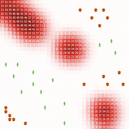
Figure 1. Snapshot of CoolWorld. Patches are coloured according to their temperature: the higher the temperature, the darker the shade of red. The white labels on each patch indicate the integral part of their temperature value. Houses are coloured in orange and walkers (represented as a person) are coloured in green.

The agents

5.6

Agents in CoolWorld are called walkers, as walking on the environment is pretty much all they do. The user can choose the number of walkers and their initial location (i.e. a certain patch). When a walker is given the opportunity to move, her behaviour is determined by the following algorithm:

• If the walker is on a patch with a house:
  • she will move to a random neighbouring patch with probability prob-leaving-home, and
  • she will stay on the same patch with probability (1 — prob-leaving-home).
• If the walker is on a patch with no house:
  • with probability prob-random-move she will move to a random neighbouring patch and,
  • with probability (1 — prob-random-move) she will explore her surroundings looking for heat. Specifically, the agent will consider the patch she is standing on together with its neighbouring patches as potential patches to be at. She will then move to one of the patches with the highest temperature within this set of potential target patches (i.e. she may stay on the same patch). Ties are resolved randomly.

The value of prob-leaving-home and prob-random-move is shared by every walker in the model. There is no restriction about the number of walkers that can stay on the same patch at any time.

Scheduling of events

5.7

Events in CoolWorld take place in discrete time-steps. In every time-step each individual walker is given the opportunity to move once.

Assessing the quality of the empirical distribution

5.8

This subsection provides guidance on how to assess the quality of a distribution obtained by simulation, i.e. how close it is to the exact one. For illustration purposes, let us assume that we are interested in studying the number of CoolWorld walkers in a house in time-step 50. The model is parameterised as follows (see Figure 2):

• Environment: The environment size is 33 patches × 33 patches and its topology is fully bounded (i.e. it does not wrap around). The temperature profile is concentrical, i.e. a patch's temperature is inversely proportional to its distance to the central patch. The distribution of houses is as shown in Figure 2.
• Walkers: There are 100 walkers and they all start at a random initial location. The value of prob-leaving-home is 0.01 and the value of prob-random-move is 0.5.

5.9

These initial conditions can be set in the implementation of CoolWorld provided in Appendix A by clicking on the button "Special conditions".

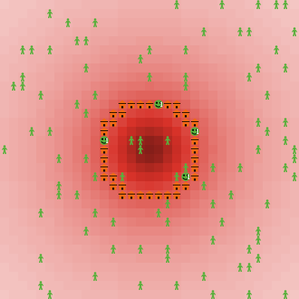
Figure 2. Snapshot of CoolWorld. Patches are coloured according to their temperature: the higher the temperature, the darker the shade of red. Houses are coloured in orange, and form a circle around the central patch. Walkers are coloured in green, and represented as a person if standing on a patch without a house, and as a smiling face if standing on a patch with a house. In the latter case, the white label indicates the number of walkers in the same house.

5.10

As argued before, given the (stochastic) initial conditions described above, the number of CoolWorld walkers in a house after 50 time-steps will follow a specific probability function that we are aiming to approximate. For that, let us assume we run 200 runs, and we plot the relative frequency of the number of walkers in a patch with a house after 50 time-steps (see Figure 3).

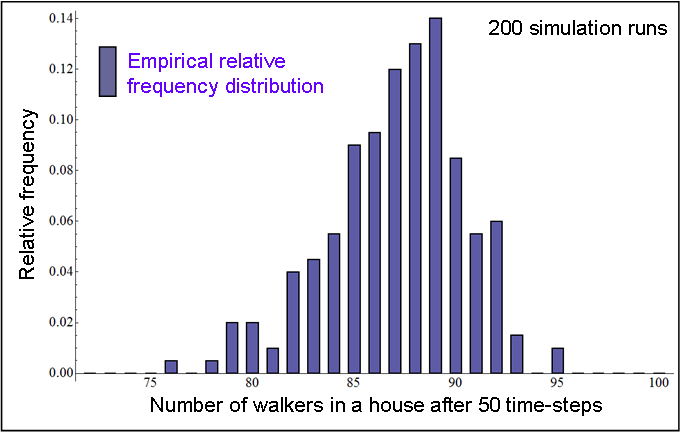
Figure 3. Relative frequency distribution of the number of walkers in a house after 50 time-steps, obtained by running CoolWorld 200 times, with the initial conditions described in the text.

5.11

Figure 3 does not provide all the information that can be extracted from the data gathered. In particular, we can plot error bars showing the standard error for each calculated frequency without hardly any effort^[6]. Standard errors give us information about the error we may be incurring when estimating the exact probabilities with the empirical frequencies. Another simple task that can be conducted consists in partitioning the set of runs into two batteries of approximately equal size and comparing the two distributions. If the two distributions are not similar, then there is no point in proceeding: we are not close to the exact distribution, so there is a need to run more simulations. Figure 4 and Figure 5 show the data displayed in Figure 3 partitioned in two batteries of 100 simulation runs, including the standard errors. Figure 4 and Figure 5 also show the exact probability function we are trying to approximate, which has been calculated using methods that are explained later in this paper.

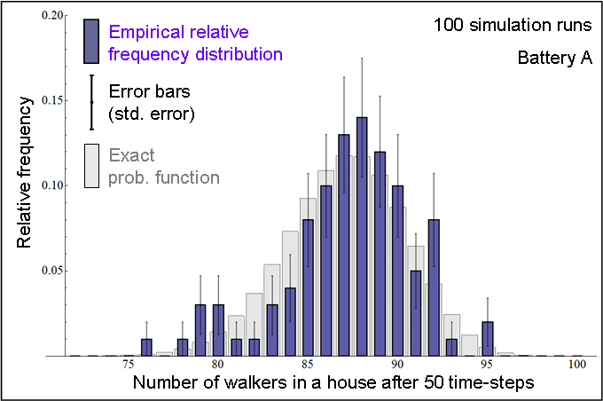
Figure 4. In blue: Relative frequency distribution of the number of walkers in a house after 50 time-steps, obtained by running CoolWorld 100 times (Battery A), with the initial conditions described in the text. In grey: Exact probability function (calculated using Markov chain analysis).

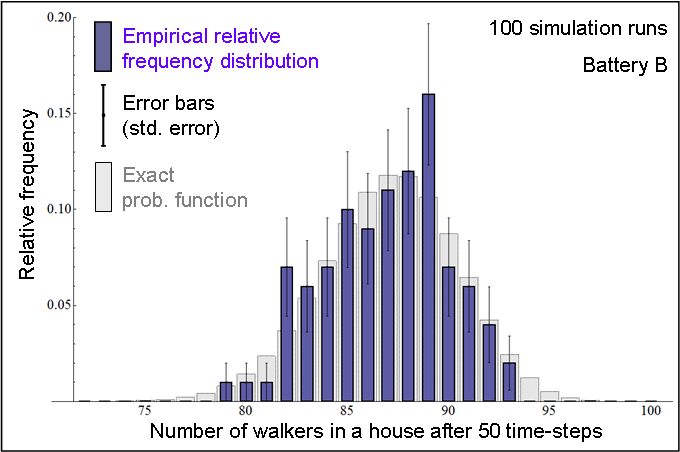
Figure 5. In blue: Relative frequency distribution of the number of walkers in a house after 50 time-steps, obtained by running CoolWorld 100 times (Battery B), with the initial conditions described in the text. In grey: Exact probability function (calculated using Markov chain analysis).

5.12

Figure 4 and Figure 5 indicate that 100 simulation runs may not be enough to obtain a satisfactory approximation to the exact probability function. On the other hand, Figure 6 and Figure 7 show that running the model 50 000 times does seem to get us close to the exact probability function. The standard error, which is inversely proportional to the square root of the sample size (i.e. the number of runs), is naturally much lower in these latter cases.

Figure 6. In blue: Relative frequency distribution of the number of walkers in a house after 50 time-steps, obtained by running CoolWorld 50 000 times (Battery A), with the initial conditions described in the text. In grey: Exact probability function (calculated using Markov chain analysis).

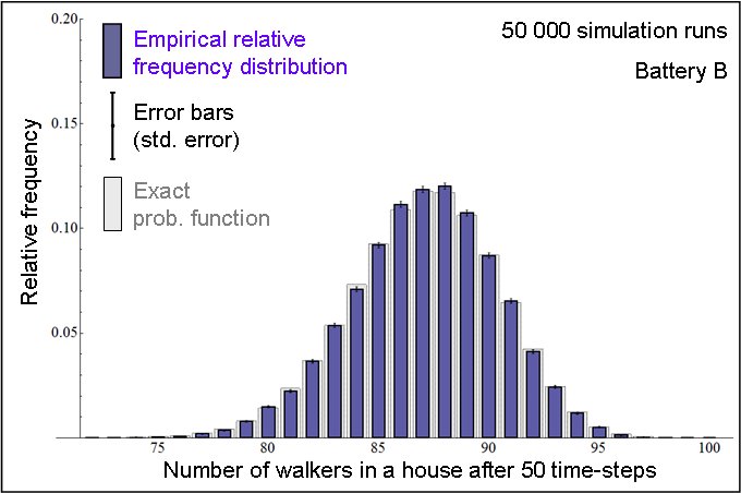
Figure 7. In blue: Relative frequency distribution of the number of walkers in a house after 50 time-steps, obtained by running CoolWorld 50 000 times (Battery B), with the initial conditions described in the text. In grey: Exact probability function (calculated using Markov chain analysis).

5.13

When, like in this example, the space of all possible outcomes in the distribution under analysis is finite (the number of walkers in a house must be an integer between 0 and 100), one can go further and calculate confidence intervals for the obtained frequencies. This is easily conducted when one realises that the exact probability function is a multinomial. Genz and Kwong (2000) show how to calculate these confidence intervals.

5.14

To conclude this section, let us emphasise that all that has been written here applies to any statistic obtained from the model and, in particular, to those that refer to various time-steps. For instance, one could study the total number of walkers that were in a house in odd time-steps in between time-steps 50 and 200. This statistic, like any other one, would follow a specific probability function that can be approximated by running the model.

Computer models as time-homogeneous Markov chains

6.1

In this section we provide guidelines to represent a particular computer model as a time-homogeneous Markov chain. This alternative representation of the model will allow us to use several simple mathematical results that will prove useful to understand the dynamics of the model. We start by describing time-homogeneous Markov chains.

What is a time-homogeneous Markov chain?

6.2

Consider a system that in time-step n = {1, 2, 3…} may be in one of a finite number of possible states S = {s₁, s₂,…, s_M}. The set S is called the state space; in this paper we only consider finite state spaces^[7]. Let the sequence of random variables X_n ∈ S represent the state of the system in time-step n. As an example, X₃ = s₉ means that at time n = 3 the system is in state s₉. The system starts at a certain initial state X₀ and moves from one state to another. The system is stochastic in that, given the present state, the system may move to one or another state with a certain probability (see Figure 8). The probability that the system moves from state i to state j in one time-step, P(X_n+1 = j | X_n = i), is denoted by p_i,j. As an example, in the Markov chain represented in Figure 8, p_4,6 equals 0 since the system cannot go from state 4 to state 6 in one single time-step. The system may also stay in the same state i, and this occurs with probability p_i,i. The probabilities p_i,j are called transition probabilities and they are often arranged in a matrix, namely the transition matrix P.

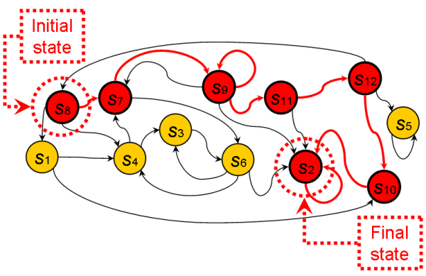
Figure 8. Schematic transition diagram of a Markov chain. Circles denote states and directed arrows indicate possible transitions between states. In this figure, circles and arrows coloured in red represent one possible path where the initial state X0 is s8 and the final state is s2.

Implicitly, our definition of transition probabilities assumes two important properties about the system:

1. The system has the Markov property. This means that the present state contains all the information about the future evolution of the system that can be obtained from its past, i.e. given the present state of the system, knowing the past history about how the system reached the present state does not provide any additional information about the future evolution of the system. Formally,

   P(X_n+1 = x_n+1 | X_n = x_n, X_n—1 = x_n—1,…, X₀ = x₀) = P(X_n+1 = x_n+1 | X_n = x_n)

2. In this paper we focus on time-homogeneous Markov chains, i.e. Markov chains with time-homogeneous transition probabilities. This basically means that transition probabilities p_i,j are independent of time, i.e. the one-step transition probability p_i,j depends on i and j but is the same at all times n. Formally,

   P(X_n+1 = j | X_n = i) = P(X_n = j | X_n—1 = i) = p_i,j

6.3

The crucial step in the process of representing a computer model as a time-homogeneous Markov chain (THMC) consists in identifying an appropriate set of state variables. A particular combination of specific values for these state variables will define one particular state of the system. Thus, the challenge consists in choosing the set of state variables in such a way that the computer model can be represented as a THMC. In other words, the set of state variables must be such that one can see the computer model as a transition matrix that unambiguously determines the probability of going from any state to any other state.

A simple random walk

6.4

Let us consider a model of a simple 1-dimensional random walk and try to see it as a THMC. In this model —which has been implemented in Applet 2— there are 17 patches in line, labelled with the integers between 1 and 17. A random walker is initially placed on one of the patches. From then onwards, the random walker will move randomly to one of the spatially contiguous patches in every time-step (staying still is not an option). Space does not wrap around, i.e. patch 1's only neighbour is patch 2.

Applet 2

Applet 2. Applet of a 1-dimensional random walk. Patches are placed in a horizontal line at the top-right corner of the applet; each of them is labelled with a red integer. Pressing the button labelled "Create Walker" allows the user to create one single random walker, by clicking with the mouse on one of the patches. Clicking on "go once" will make the random walker move once, while "go" asks the random walker to move indefinitely. The plot beneath the patches shows the time series of the random walker's position. Patches are coloured in shades of blue according to the number of times that the random walker has visited them: the higher the number of visits, the darker the shade of blue. This applet has been created with NetLogo 4.0 (Wilensky 1999) and its source code can be downloaded here.

6.5

The model shown in Applet 2 can be easily represented as a THMC by choosing the agent's position (e.g. the number of the patch she is standing on) as the only state variable. To be sure, note that defining the state of the system in this way, it is true that there is a fixed probability of going from any state to any other state, independent of time. Figure 9 shows the transition diagram of this THMC.

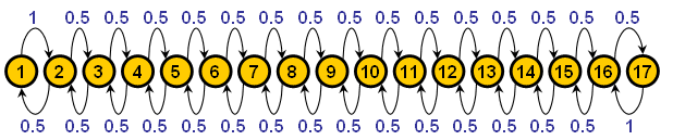
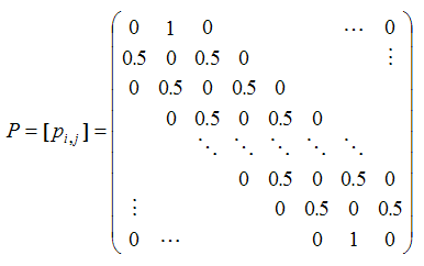
Figure 9. Transition diagram of the model shown in Applet 2. Each yellow circle represents a state of the system, with the number inside denoting the patch number. Arrows between states show possible transitions between states. Every arrow has a blue label that indicates the probability with which that transition takes place.

6.6

The transition matrix P = [p_i,j] corresponding to the model shown in Applet 2 is:

(1)

Where, as explained above, p_i,j is the probability P(X_n+1 = j | X_n = i) that the system will be in state j in the following time-step, knowing that it is currently in state i.

CoolWorld as a THMC

6.7

CoolWorld can be represented as a THMC by defining the state of the system as a vector containing the number of walkers in each patch. It is then clear that, once the model has been parameterised, and given a particular state of the system, the probability function over states of the system for the following time-step is completely determined.

Simulation models in the literature as THMCs

6.8

Appendix B shows 10 famous models in the social simulation literature that can be usefully represented as time-homogeneous Markov chains. This appendix also includes the analysis of each of these models using the concepts that we explain below.

Transient distributions of finite THMCs

7.1

The analysis of the dynamics of THMCs is usually divided into two parts: transient dynamics (finite time) and asymptotic dynamics (infinite time). The transient behaviour is characterised by the distribution of the state of the system X_n for a fixed time-step n ≥ 0. The asymptotic behaviour (see sections 8-10) is characterised by the limit of the distribution of X_n as n goes to infinity, when this limit exists.

7.2

This section explains how to calculate the transient distribution of a certain THMC, i.e. the distribution of X_n for a fixed n ≥ 0. In simple words, we are after a vector a⁽ⁿ⁾ containing the probability of finding the process in each possible state in time-step n. Formally, a⁽ⁿ⁾ = [a₁⁽ⁿ⁾, … , a_M⁽ⁿ⁾] , where a_i⁽ⁿ⁾ = P(X_n = i), denotes the distribution of X_n for a THMC with M possible states. In particular, a⁽⁰⁾ denotes the initial distribution over the state space, i.e. a_i⁽⁰⁾ = P(X₀ = i). Note that there is no problem in having uncertain initial conditions, i.e. probability functions over the space of possible inputs to the model.

It can be shown that one can easily calculate the transient distribution in time-step n, simply by multiplying the initial conditions by the n-th power of the transition matrix P.

Proposition 1. a⁽ⁿ⁾ = a⁽⁰⁾ · Pⁿ.

Thus, the elements p⁽ⁿ⁾_i,j of Pⁿ represent the probability that the system is in state j after n time-steps having started in state i, i.e. p⁽ⁿ⁾_i,j = P(X_n = j | X₀ = i). A straightforward corollary of Proposition 1 is that a^(n+m) = a⁽ⁿ⁾ · P^m.

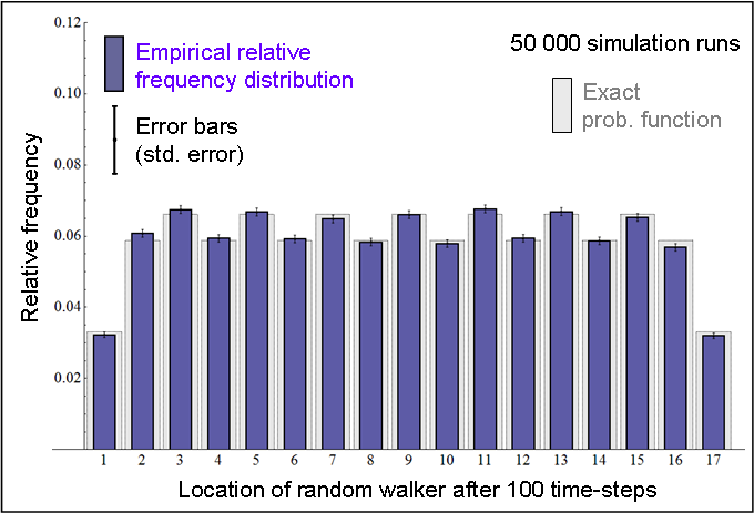
As an example, let us consider the 1-dimensional random walk implemented in Applet 2. Imagine that the random walker starts at a random initial location, i.e. a⁽⁰⁾ = [1/17, …, 1/17]. The exact distribution of the walker's position in time-step 100 would then be a⁽¹⁰⁰⁾ = a⁽⁰⁾ · P¹⁰⁰. This distribution is represented in Figure 10, together with an empirical distribution obtained by running the model 50 000 times.

Figure 10. Probability function of the position of Applet 2's random walker in time-step 100, starting at a random initial location.

7.3

Let us see a more sophisticated example with CoolWorld. Consider a model parameterised as described in paragraph 5.8 (see Figure 2), but instead of having 100 walkers, we place a single walker at one of the corners of the environment. With these settings, there are 33 × 33 possible states, corresponding to the 33 × 33 patches where the walker may be. The temperature profile and the distribution of houses fully determine the transition matrix. Thus, the initial state is a⁽⁰⁾ = [1, 0 … 0], which denotes that the walker is on the patch at the corner (this is state 1) with certainty. Multiplying a⁽⁰⁾ by the transition matrix repeatedly we can obtain the exact probability a_i⁽ⁿ⁾ = P(X_n = i) that the walker is on any patch i at any time n. This is illustrated in figure 11, which shows the transient distributions of this model as time goes by.

Figure 11. Transient distributions of the location of a single walker in a CoolWorld model where the temperature profile and the distribution of houses are as described in paragraph 5.8. The height of each patch denotes the relative probability that the walker is on the patch in any given time-step. In other words, the plot uses height to represent a(n) for each time-step n.

7.4

Having obtained the probability function over the states of the system for any fixed n, namely the probability mass function of X_n, it is then straightforward to calculate the distribution of any statistic that can be extracted from the model. As argued in the previous sections, the state of the system fully characterises it, so any statistic that we obtain about the computer model in time-step n must be, ultimately, a function of {X₀, X₁, …, X_n}.

7.5

As an example, to calculate the probability that the solitary walker in CoolWorld is in a house in time-step 50, one would simply add the elements of a⁽⁵⁰⁾ corresponding to the states where the walker is in a house. Similarly, if we wanted to calculate e.g. the average time that the walker spends in a house from time-step 0 to time-step 50, we would proceed analogously, but using the 51 vectors a^(t), t = {0, 1,…,50}. The analysis of models with any number of walkers is not significantly more complex; in particular, the exact probability functions shown in Figures 4, 5, 6 and 7 were calculated using the method explained in this section.

7.6

Admittedly, the transition matrix of most computer models cannot be easily derived, or it is unfeasible to operate with it. Nonetheless, this apparent drawback is not as important as one might expect. As we shall see below, it is often possible to infer many properties of a THMC even without knowing the exact values of its transition matrix, and these properties can yield useful insights about the dynamics of the associated process. Knowing the exact values of the transition matrix allows us to calculate the exact transient distributions using Proposition 1; this is desirable but not critical, since we can always approximate these distributions by conducting many simulation runs, as explained in section 5.

Important concepts

8.1

This section presents some basic concepts that will prove useful to analyse the dynamics of computer models. The notation used here follows the excellent book on stochastic processes written by Kulkarni (1995).

Definition 1: Accessibility

8.2

A state j is said to be accessible from state i if starting at state i there is a chance that the system may visit state j at some point in the future. By convention, every state is accessible from itself. Formally, a state j is said to be accessible from state i if for some n ≥ 0, p⁽ⁿ⁾_i,j > 0.

Note that j is accessible from i ≠ j if and only if there is a directed path from i to j in the transition diagram. In that case, we write i→j. If i→j we also say that i leads to j. As an example, in the THMC represented in Figure 8, s₂ is accessible from s₁₂ but not from s₅. Note that the definition of accessibility does not depend on the actual magnitude of p⁽ⁿ⁾_i,j , only on whether it is exactly zero or strictly positive.

Definition 2: Communication

8.3

A state i is said to communicate with state j if i→j and j→i.

If i communicates with j we also say that i and j communicate and write i↔j. As an example, note that in the simple random walk presented in paragraph 6.4 (see Applet 2) every state communicates with every other state. It is worth noting that the relation "communication" is transitive, i.e.

{i↔j , j↔k} ⇒ i↔k.

Definition 3: Communicating class

8.4

A set of states C ⊂ S is said to be a communicating class if:

• Any two states in the communicating class communicate with each other. Formally,

  {i ∈ C, j ∈ C } ⇒ i↔j

• The set C is maximal, i.e. no strict superset of a communicating class can be a communicating class. Formally,

  {i ∈ C, i↔j} ⇒ j ∈ C

As an example, note that in the simple random walk presented in paragraph 6.4 there is one single communicating class that contains all the states. Similarly, any CoolWorld model where prob-leaving-home ∈ (0, 1) and prob-random-move ∈ (0, 1) has one single communicating class containing all the possible states. In the THMC represented in Figure 8 there are 4 communicating classes: {s₂}, {s₅}, {s₁₀}, {s₁, s₃, s₄, s₆, s₇, s₈, s₉, s₁₁, s₁₂}.

Definition 4: Closed communicating class (i.e. absorbing class). Absorbing state.

8.5

A communicating class C is said to be closed if no state within C leads to any state outside C. Formally, a communicating class C is said to be closed if i ∈ C and j ∉ C implies that j is not accessible from i.

Note that once a Markov chain visits a closed communicating class, it cannot leave it. Hence we will sometimes refer to closed communicating classes as "absorbing classes". This latter term is not standard in the literature, but we find it useful here for explanatory purposes. Note that if a Markov chain has one single communicating class, it must be closed.

As an example, note that the communicating classes {s₁₀} and {s₁, s₃, s₄, s₆, s₇, s₈, s₉, s₁₁, s₁₂} in the THMC represented in Figure 8 are not closed, as they can be abandoned. On the other hand, the communicating classes {s₂} and {s₅} are indeed closed, since they cannot be abandoned. When a closed communicating class consists of one single state, this state is called absorbing. Thus, s₂ and s₅ are absorbing states. Formally, state i is absorbing if and only if p_i,i = 1 and p_i,j = 0 for i ≠ j.

Proposition 2. Decomposition Theorem (Chung, 1960)

8.6

The state space S of any Markov chain can be uniquely partitioned as follows:

S = C₁ ∪ C₂ ∪ … ∪ C_k ∪ T where C₁, C₂, …, C_k are closed communicating classes, and T is the union of all other communicating classes.

Note that we do not distinguish between non-closed communicating classes: we lump them all together into T. Thus, the unique partition of the THMC represented in Figure 8 is S = {s₂} ∪ {s₅} ∪ {s₁, s₃, s₄, s₆, s₇, s₈, s₉, s₁₀, s₁₁, s₁₂}. Any CoolWorld model where prob-leaving-home ∈ (0, 1) and prob-random-move ∈ (0, 1) has one single (closed) communicating class C₁ containing all the possible states, i.e. S ≡ C₁. Similarly, all the states in the simple random walk presented in paragraph 6.4 belong to the same (closed) communicating class.

Definition 5: Irreducibility

8.7

A Markov chain is said to be irreducible if all its states belong to a single closed communicating class; otherwise it is called reducible. Thus, the simple random walk presented in paragraph 6.4 is irreducible, but the THMC represented in Figure 8 is reducible.

Definition 6: Transient and recurrent states

8.8

A state i is said to be transient if, given that we start in state i, there is a non-zero probability that we will never return back to i. Otherwise, the state is called recurrent. A Markov chain starting from a recurrent state will revisit it with probability 1, and hence revisit it infinitely often. On the other hand, a Markov chain starting from a transient state has a strictly positive probability of never coming back to it. Thus, a Markov chain will visit any transient state only finitely many times; eventually, transient states will not be revisited anymore.

Definition 7: Periodic and aperiodic states. Periodic and aperiodic communicating classes

8.9

A state i has period d if any return to state i must occur in multiples of d time-steps. If d = 1, then the state is said to be aperiodic; otherwise (d > 1), the state is said to be periodic with period d. Formally, state i's period d is the greatest common divisor of the set of integers n > 0 such that p⁽ⁿ⁾_i,i > 0. For our purposes, the concept of periodicity is only relevant for recurrent states.

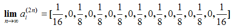
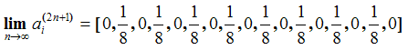
As an example, note that every state in the simple random walk presented in paragraph 6.4 is periodic with period 2. On the other hand, every state in any CoolWorld model where prob-leaving-home ∈ (0, 1) and prob-random-move ∈ (0, 1) is aperiodic.

An interesting and useful fact is that if i↔j , then i and j must have the same period (see theorem 5.2. in Kulkarni (1995)). In particular, note that if p_i,i > 0 for any i, then the communicating class to which i belongs must be aperiodic. Thus, it makes sense to qualify communicating classes as periodic with period d, or aperiodic. A closed communicating class with period d can return to its starting state only at times d, 2d, 3d, …

8.10

The concepts presented in this section will allow us to analyse the dynamics of any finite Markov chain. In particular, we will show that, given enough time, any finite Markov chain will necessarily end up in one of its closed communicating classes (i.e. absorbing classes).

Limiting behaviour of THMCs

9.1

This section is devoted to characterising the limiting behaviour of a THMC, i.e. studying the convergence (in distribution) of X_n as n tends to infinity. Specifically, we aim to study the behaviour of a_i⁽ⁿ⁾ = P(X_n = i) as n tends to infinity. From Proposition 1 it is clear that analysing the limiting behaviour of Pⁿ would enable us to characterise a_i⁽ⁿ⁾. There are many introductory books in stochastic processes that offer clear and simple methods to analyse the limiting behaviour of THMCs when the transition matrix P is tractable (see e.g. chapter 5 in Kulkarni (1999), chapters 2-4 in Kulkarni (1995), chapter 3 in Janssen and Manca (2006) or the book chapter written by Karr (1990)). Nonetheless, we focus here on the general case, where operating with the transition matrix P may be computationally unfeasible.

General dynamics

9.2

The first step in the analysis of any THMC consists in identifying all the closed communicating classes, so we can partition the state space S as indicated by the decomposition theorem (see Proposition 2). The following proposition (Theorems 3.7 and 3.8 in Kulkarni (1995)) reveals the significance of this partition:

Proposition 3. General dynamics of finite THMCs.

9.3

Consider a finite THMC that has been partitioned as indicated in Proposition 2. Then:

1. All states in T (i.e. not belonging to a closed communicating class) are transient.
2. All states in C_v (i.e. in any closed communicating class) are recurrent; v ∈ {1, 2, …, k}.

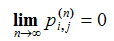
Proposition 3 states that sooner or later the THMC will enter one of the absorbing classes and stay in it forever. Formally, for all i ∈ S and all j ∈ T: , i.e. the probability of finding the process in a state belonging to a non-closed communicating class goes to zero as n goes to infinity. Naturally, if the initial state already belongs to an absorbing class C_v, then the chain will never abandon such a class. Formally, for all i ∈ C_v and all j ∉ C_v: p⁽ⁿ⁾_i,j = 0 for all n ≥ 0. We provide now two examples to illustrate the usefulness of Proposition 3.

THMC represented in Figure 8

9.4

This THMC has only two absorbing classes: {s₂} and {s₅}. Thus, the partition of the state space is: S = {s₂} ∪ {s₅} ∪ {s₁, s₃, s₄, s₆, s₇, s₈, s₉, s₁₀, s₁₁, s₁₂}. Hence, applying Proposition 3 we can state that the process will eventually end up in one of the two absorbing states, s₂ or s₅. The probability of ending up in one or the other absorbing state depends on the initial conditions a⁽⁰⁾ (and on the actual numbers p_i,j in the transition matrix, of course). Slightly more formally, the limiting distribution of X_n exists, but it is not unique, i.e. it depends on the initial conditions.

CoolWorld

9.5

Consider any CoolWorld model with at least one house, with prob-random-move strictly positive and with prob-leaving-home exactly equal to 0. Under such conditions, every state where all walkers are in a house is absorbing (and there are no more absorbing classes). Thus, any CoolWorld simulation satisfying the mentioned conditions will necessarily end up with all walkers in a house, regardless of the temperature profile or the distribution of houses. In particular, if there is one single house, then sooner or later every walker will end up in the only house. The reader may want to corroborate this fact using the applet in Appendix A.

Dynamics within absorbing classes

9.6

The previous subsection (i.e. "General Dynamics") has explained that any simulation run will necessarily end up in a certain absorbing class; this subsection characterises the dynamics of a THMC that is already "trapped" in an absorbing class. This is precisely the analysis of irreducible Markov chains, since irreducible Markov chains are, by definition, Markov chains with one single closed communicating class (see Definition 5). In other words, one can see any THMC as a set of transient states T plus a finite number of irreducible Markov sub-chains.

9.7

Irreducible THMCs behave significantly different depending on whether they are periodic or not. The following subsections characterise these two cases.

Irreducible and aperiodic THMCs

9.8

Irreducible and aperiodic THMCs are often called ergodic. In these processes the probability function of X_n approaches a limit as n tends to infinity. This limit is called the limiting distribution, and is denoted here by π. Formally, the following limit exists and is unique (i.e. independent of the initial conditions a_i⁽⁰⁾):

9.9

Thus, in ergodic THMCs the probability of finding the system in each of its states in the long run is strictly positive and independent of the initial conditions (Theorems 3.7 and 3.15 in Kulkarni (1995)). As previously mentioned, calculating such probabilities may be unfeasible, but we can estimate them sampling many simulation runs at a sufficiently large time-step.

9.10

Importantly, in ergodic THMCs the limiting distribution π coincides with the occupancy distribution π*, which is the long-run fraction of the time that the THMC spends in each state^[8]. Naturally, the occupancy distribution π* is also independent of the initial conditions. Thus, in ergodic THMCs, running just one simulation for long enough (which enables us to estimate π*) will serve to estimate π just as well.

9.11

The question that comes to mind then is: How long is long enough? i.e. when will I know that the empirical distribution obtained by simulation resembles the limiting distribution π? Unfortunately there is no answer for that. The silver lining is that knowing that the limiting and the occupancy distribution coincide, that they must be stable in time, and that they are independent of the initial conditions, enables us to conduct a wide range of tests that may tell us when it is certainly not long enough. For example, we can run a battery of simulations and study the empirical distribution over the states of the system across samples as time goes by. If the distribution is not stable, then we have not run the model for long enough. Similarly, since the occupancy distribution is independent of the initial conditions, one can run several simulations with widely different initial conditions, and compare the obtained occupancy distributions. If the empirical occupancy distributions are not similar, then we have not run the model for long enough. Many more checks can be conducted.

9.12

Admittedly, when analysing a computer model one is often interested not so much in the distribution over the possible states of the system, but rather in the distribution of a certain statistic. The crucial point is to realise that if the statistic is a function of the state of the system (and all statistics that can be extracted from the model are), then the limiting and the occupancy distributions of the statistic exist, coincide and are independent of the initial conditions.

9.13

To illustrate this, we present some results with CoolWorld parameterised as described in paragraph 5.8. An example of a potentially interesting statistic in CoolWorld is the number of walkers in each patch. The first step is to ensure that the THMC is irreducible and aperiodic. Note that since prob-random-move and prob-leaving-home are in the interval (0, 1), every state communicates with every other state, i.e. the THMC is irreducible. Identifying one state i such that p_i,i > 0 will guarantee that the THMC is also aperiodic (see Definition 7). An example of such an aperiodic state is any state where every walker is in a house. Thus, the parameterised model has a unique limiting distribution over all the possible states, independent of the initial conditions (i.e. independent of the initial location of the walkers); consequently, the number of walkers in each of the patches also has a unique limiting distribution which is independent of the initial conditions and coincides with its occupancy distribution, i.e. in the limit as n goes to infinity the probability of having k walkers in any particular patch coincides with the proportion of the time that there are k walkers in the patch.

9.14

This is illustrated in Figures 12 and 13. Figure 12 shows the average number of walkers in each patch over time-steps 0 to 10 000, calculated with one single run (i.e. an estimation of the mean of the occupancy distribution for each patch, assuming 10 000 time-steps are enough). On the other hand, Figure 13 shows the average number of walkers in each patch in time-step 1000, calculated over 1000 simulation runs (i.e. an estimation of the mean of the limiting distribution for each patch, assuming 1000 time-steps are enough). Without getting into details, note that the exact value of the long-run expected number of walkers in each patch was shown (in relative terms) in Figure 11 (the frame labelled with ∞).

Figure 12. Average number of walkers in each patch over time-steps 0 to 10 000 calculated with one single run (i.e. an estimation of the mean of the occupancy distribution for each patch, assuming 10 000 time-steps are enough) in a CoolWorld model parameterised as described in paragraph 5.8.

Figure 13. Average number of walkers in each patch in time-step 1000, calculated over 1000 simulation runs (i.e. an estimation of the mean of the limiting distribution for each patch, assuming 1000 time-steps are enough) in a CoolWorld model parameterised as described in paragraph 5.8.

9.15

Given the importance of irreducible and aperiodic THMCs, we conclude this subsection providing some sufficient conditions that guarantee that a finite THMC is irreducible and aperiodic (i.e. ergodic):

Proposition 4. Sufficient conditions for irreducibility and aperiodicity.

1. If it is possible to go from any state to any other state in one single time-step (p_i,j > 0 for all i ≠ j) and there are more than 2 states, then the THMC is irreducible and aperiodic.
2. If it is possible to go from any state to any other state in a finite number of time-steps (i↔j for all i ≠ j), and there is at least one state in which the system may stay for two consecutive time-steps (p_i,i > 0 for some i), then the THMC is irreducible and aperiodic.
3. If there exists a positive integer n such that p⁽ⁿ⁾_i,j > 0 for all i and j, then the THMC is irreducible and aperiodic (Janssen and Manca 2006, p. 107).

Irreducible and periodic THMCs

9.16

In contrast with aperiodic THMCs, the probability distribution of X_n in periodic THMCs does not approach a limit as n tends to infinity. Instead, in an irreducible THMC with period d, as n tends to infinity, X_n will in general cycle through d probability functions depending on the initial distribution.

9.17

As an example, consider the simple random walk presented in paragraph 6.4 (which is irreducible and periodic, with period 2), and assume that the random walker starts at patch number 1 (i.e. X₀ = 1). Given these settings, it can be shown that

9.18

In particular, the limits above show that the random walker cannot be at a patch with an even number in any even time-step, and he cannot be at a patch with an odd number in any odd time-step. In contrast, if the random walker started at patch number 2 (i.e. X₀ = 2), then the limits above would be interchanged.

9.19

Fortunately, every irreducible (periodic or aperiodic) THMC does have a unique occupancy distribution π*, independent of the initial conditions (see Theorem 5.19 in Kulkarni (1999)). In our particular example, this is:

9.20

Thus, the long-run fraction of time that the system spends in each state in any irreducible THMC is unique (i.e. independent of the initial conditions). This is a very useful result, since any statistic which is a function of the state of the system will also have a unique occupancy distribution independent of the initial conditions. As explained before, this occupancy distribution can be approximated with one single simulation run, assuming it lasts for long enough. The reader may want to corroborate this using Applet 2.

Absorbing states and stochastic stability

10.1

This last section deals with the analysis of models with absorbing states. Many computer models in the social simulation literature can be represented as (reducible) THMCs with several absorbing states, and with no other absorbing classes (e.g. for most parameterisations: Schelling's (1971) model of spatial segregation, Miller and Page's (2004) standing ovation model, Axelrod and Bennett's (1993) model of competing bimodal coalitions, and Kinnaird's (1946) truels). Thus, the partition of the state space in these models follows the pattern: S = {abs₁} ∪ {abs₂} ∪ … ∪ {abs_k} ∪ T, where abs₁, abs₂, …, abs_k are absorbing states, and T is the union of all non-closed communicating classes. This section analyses models that follow this pattern.

10.2

If the model has only one absorbing state (i.e. S = {abs₁} ∪ T), the analysis is straightforward. The system will eventually end up in the absorbing state with probability 1 regardless of the initial conditions, i.e.

10.3

If, on the other hand, there are several absorbing states, then Proposition 3 states that the system will eventually reach one of these absorbing states (i.e. the set formed by all absorbing states is reached with probability 1). The probability of ending up in any one particular absorbing state depends on the initial conditions. In this section we study the robustness of each of these absorbing states to small perturbations. In evolutionary models these perturbations may derive from mutation processes; in cultural models they may derive from experimentation. In any case, perturbations are understood here as some sort of noise that enables the system to make moves between states that were not possible in the unperturbed model. In particular, it is assumed here that escape from previously absorbing states is possible due to perturbations. Thus, when noise is added to these models the partition of their state space changes significantly. Most often, the inclusion of noise makes the THMC irreducible and aperiodic (i.e. ergodic), or uni-reducible. Uni-reducible THMCs have one single absorbing class (i.e. S = C₁ ∪ T); we assume here that this absorbing class is aperiodic. In both these cases (ergodic THMCs and uni-reducible THMCs with an aperiodic absorbing class) there is a unique limiting distribution independent of the initial conditions. As explained in section 9, this limiting distribution coincides with the occupancy distribution.

10.4

Hence, the inclusion of (even tiny levels of) noise may alter the dynamics of these systems dramatically. In general, for low enough levels of noise we find the unique limiting distribution concentrated on the neighbourhoods of the previously absorbing states (PAS). The lower the noise, the higher the concentration around the PASs.

10.5

The interesting point is that when noise is added, it is often the case that some of the absorbing states that could be reached with arbitrarily large probability in the unperturbed model are observed with very low probability in the model with noise. In other words, the limiting distribution of the model with noise may concentrate on some of the PASs much more than on others. In the limit as the noise goes to zero, it is often the case that only some of the PASs remain points of concentration. These are called stochastically stable states (Foster and Young 1990; Young 1993; Ellison 2000). Stochastically stable states are important because they constitute the set of states where the slightly perturbed system spends a significant proportion of time in the long-term. Furthermore, the set of stochastically stable states is generally the same for a surprisingly wide range of structurally different types of noise (see Young 1993). Young (1993) provides a general method to identify stochastically stable states by solving a series of shortest path problems in a graph. Ellison (2000) complements Young's approach with another method which is not always conclusive, but it is often easier to apply and more intuitive. For an overview of this part of the literature, see Vega-Redondo (2003, section 12.6), who provides an excellent account of the basic concepts and techniques to analyse perturbed Markov processes.

10.6

The remaining of this section is devoted to illustrate the concept of stochastic stability with an example of a simple model where two reinforcement learners play a 2 × 2 game. (A more sophisticated version of this model has been analysed by Macy and Flache (2002), Flache and Macy (2002), and Izquierdo et al. (2007; 2008)).

A model of reinforcement learning in 2x2 games

10.7

Reinforcement learners use their experience to choose or avoid certain actions based on the observed consequences. Actions that led to satisfactory outcomes (i.e. outcomes that met or exceeded aspirations) in the past tend to be repeated in the future, whereas choices that led to unsatisfactory experiences are avoided.

The formal model

10.8

In the model presented here (and implemented in Applet 3) there are two reinforcement learners playing a Prisoner's Dilemma repeatedly. The Prisoner's Dilemma is a two-person game where each player can either cooperate (C) or defect (D). For each player r, the payoff when they both cooperate (u_r(C, C) = R_r, for Reward) is greater than the payoff obtained when they both defect (u_r(D, D) = P_r, for Punishment); if one cooperates and the other defects, the cooperator obtains S_r (Sucker), whereas the defector receives T_r (Temptation). The dilemma comes from the fact that, individually, each player is better off defecting given any of her counterpart's choices (T_r > R_r and P_r > S_r; r = 1, 2), but they both obtain a greater payoff when they both cooperate than when they both defect (R_r > P_r; r = 1, 2).

Applet 3

Applet3. A model of reinforcement learning for 2 × 2 games. The white square on the top right is a representation of the state space, with player 1's propensity to cooperate in the vertical axis and player 2's propensity to cooperate in the horizontal axis. Thus, each patch in this square corresponds to one state. The red circle represents the current state of the system and its label (CC, CD, DC, or DD) denotes the last outcome that occurred. Patches are coloured in shades of blue according to the number of times that the system has visited the state they represent: the higher the number of visits, the darker the shade of blue. The plot beneath the representation of the state space shows the time series of both players' propensity to cooperate. This applet has been created with NetLogo 4.0 (Wilensky 1999) and its source code can be downloaded here.

10.9

In this model, each player r has a certain propensity to cooperate p_r,C and a certain propensity to defect p_r,D; in Applet 3 these propensities are always multiples of 1/16. In the absence of noise, players cooperate with probability p_r,C and defect with probability p_r,D, but they may also suffer from 'trembling hands' (Selten 1975), i.e. after having decided which action to undertake, each player r may select the wrong action with probability trembling-hands-noise.

10.10

The revision of propensities takes place following a reinforcement learning approach: players increase their propensity of undertaking a certain action if it led to payoffs that at least met their aspiration level A_r, and decrease this propensity otherwise. Specifically, if a player r receives a payoff greater or equal to her aspiration threshold A_r, she increments the propensity of conducting the selected action in 1/16 (within the natural limits of probabilities). Otherwise she decreases this propensity in 1/16.

10.11

Mathematically, after outcome oⁿ = {action₁, action₂} in time-step n, each player r updates her propensity of undertaking the selected action action_r as follows (within the natural limits of probabilities):

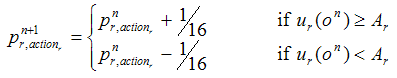
where pⁿ_r,action is player r's propensity to undertake action action_r in time-step n, and u_r(oⁿ) is the payoff obtained by player r in time-step n, having experienced outcome oⁿ. The updated propensity for the action not selected derives from the constraint that propensities must add up to one. Note that this model can be represented as a THMC by defining the state of the system as a vector containing both players' propensity to cooperate, i.e. [p_1,C , p_2,C]. The following subsections analyse models where T_r > R_r > P_r > A_r > S_r, r = 1, 2.

Analysis of the model without noise

10.12

The model with trembling-hands-noise = 0 has two absorbing states: one where both players cooperate with probability 1 (denoted by abs_C) and another one where both players defect with probability 1 (denoted by abs_D). Thus, S = {abs_C} ∪ {abs_D} ∪ T. Starting from any non-absorbing state with p_r,C > 0 (r = 1, 2), there is a strictly positive probability of ending up in each of the two absorbing states. Naturally, these probabilities depend on the initial conditions. As an example, if the initial state is [p_1,C , p_2,C] = [0.875 , 0.625], then the system will end up in abs_C with probability 0.635 and in abs_D with probability 0.365. Figure 14 shows the transient distributions of this model as time goes by.

Figure 14. Transient distributions of the reinforcement learning model without trembling hands noise. Each patch represents a certain state of the system [p1,C , p2,C]. The closest patch to the vertical axis on the left represents the state where both players' propensity to cooperate is 0. The axis departing away from us from the origin denotes player 1's propensity to cooperate. The other axis (coming towards us) denotes player 2's propensity to cooperate. The height of each patch denotes the probability that the system is on the state represented by the patch in any given time-step. In other words, the plot uses height to represent the distribution of Xn for each time-step n.

Analysis of the model with noise

10.13

In contrast with the unperturbed model, the model with trembling-hands-noise ≠ 0 is uni-reducible with no absorbing states. It can be shown that there is one single (aperiodic) absorbing class C₁ containing all the states where players' propensities to cooperate are the same, i.e. p_1,C = p_2,C. Thus, S = C₁ ∪ T, and the model has a unique limiting distribution independent of the initial state. Figure 15 shows the transient distributions of this model with trembling-hands-noise = 0.1 as time goes by, and the limiting distribution.

Figure 15. Transient distributions of the reinforcement learning model with trembling hands noise equal to 0.1. Each patch represents a certain state of the system [p1,C , p2,C]. The closest patch to the vertical axis on the left represents the state where both players' propensity to cooperate is 0. The axis departing away from us from the origin denotes player 1's propensity to cooperate. The other axis (coming towards us) denotes player 2's propensity to cooperate. The height of each patch denotes the probability that the system is on the state represented by the patch in any given time-step. In other words, the plot uses height to represent the distribution of Xn for each time-step n.

10.14

The limiting distribution of the noisy model (which is independent of the initial conditions) is concentrated on the uncooperative PAS [p_1,C , p_2,C] = [0, 0]. It can be shown that the uncooperative PAS is the only stochastically stable state. Thus, even though the unperturbed model could end up in the cooperative PAS [p_1,C , p_2,C] = [1, 1] with arbitrarily large probability, the long-run fraction of time that the perturbed system spends in the cooperative PAS tends to 0 as the noise tends to 0, regardless of the initial conditions. In the limit as the noise tends to 0, only the uncooperative PAS would be observed.

10.15

Intuitively, note that when the system is at the cooperative PAS (or in its proximities), one single (possibly mistaken) defection is enough to lead the system away from it. On the other hand, when the system is at the uncooperative PAS at [0 , 0] (or nearby), one single (possibly mistaken) cooperation will not make the system move away from the uncooperative PAS. Only a coordinated mutual cooperation (which is highly unlikely at the PAS at [0, 0] and in its proximities) will make the system move away from this uncooperative PAS. This makes the uncooperative PAS at [0, 0] much more robust to occasional mistakes made by the players when selecting their strategies than the cooperative PAS at [1, 1], as illustrated in Figure 15.

Summary

11.1

This paper has shown that many computer simulation models can be usefully represented as time-homogenous Markov chains. Representing a computer model within the framework of Markov chains can yield insights about the dynamics of the model that are not evident by exploring individual runs of the model only. This paper has focused on the analysis of Markov chains with finite state space.

11.2

The first step to analyse a model as a Markov chain consists in finding an appropriate definition of the state of the system. This definition must be such that one can see the computer model as a transition matrix that unambiguously determines the probability of going from any state to any other state. The next step consists in identifying all the closed communicating (i.e. absorbing) classes in the model C_v (v ∈ {1, 2, …, k}). This allows us to partition the state space of the Markov chain as the union of all the closed communicating classes C₁, C₂, …, C_k in the model plus another class T containing all the states that belong to non-closed communicating classes.

11.3

Having conducted this partition, the analysis of the dynamics of the model is straightforward: all states in T (i.e. in any finite communicating class that is not closed) are transient, whereas all states in C_v (i.e. in any finite closed communicating class) are recurrent. In other words, sooner or later any simulation run will enter one of the absorbing classes C_v and stay in it forever. Thus, the following step consists in characterising the dynamics of the system within each of these absorbing classes.

11.4

Once the system has entered a certain absorbing class C_v, it will remain in it forever exhibiting a unique conditional^[9] occupancy distribution π_v* over the set of states that compose C_v. This conditional occupancy distribution π_v* denotes the (strictly positive) long-run fraction of the time that the system spends in each state of C_v given that the system has entered C_v. Importantly, the conditional occupancy distribution π_v* is the same regardless of the specific state through which the system entered C_v.

11.5

Some absorbing classes are periodic and some are aperiodic. Aperiodic absorbing classes have a unique conditional limiting distribution π_v denoting the long-run (strictly positive) probability of finding the system in each of the states that compose C_v given the system has entered C_v. This conditional limiting distribution π_v coincides with the conditional occupancy distribution π_v* and, naturally, is also independent of the specific state through which the system entered C_v. In contrast with aperiodic absorbing classes, periodic absorbing classes do not generally have a unique limiting distribution; instead, they cycle through d probability functions depending on the specific state through which the system entered C_v (where d denotes the period of the periodic absorbing class).

11.6

The type of analysis explained in this paper is useful even if —as in most cases— the probability functions described above cannot be derived analytically. These probability functions can always be approximated with any degree of accuracy by running the computer model several times. The important point is that realising that such probability functions exist, and knowing when and how they depend on the initial conditions, can provide useful insights about the dynamics of many computer models. This fact has been illustrated in this paper by analysing 10 well-known models in the social simulation literature.

Acknowledgements

The authors have benefited from the financial support of the Spanish Ministry of Education and Science (projects DPI2004-06590, DPI2005-05676 and TIN2008-06464-C03-02) and of the JCyL (project BU034A08). We are also very grateful to Nick Gotts, Bruce Edmonds, Gary Polhill, Cesáreo Hernández and Seth Tisue for many extremely useful discussions.

Notes

¹A formal model is a model expressed in a formal system (Cutland 1980). A formal system consists of a formal language and a deductive apparatus (a set of axioms and inference rules). Formal systems are used to derive new expressions by applying the inference rules to the axioms and/or previously derived expressions in the same system.

²Note that simulations of stochastic models are actually using pseudorandom number generators, which are deterministic algorithms that require a seed as an input.

³The mere fact that the model has been implemented and can be run in a computer is a proof that the model is formal (Suber 2007).

⁴As a matter of fact, strictly speaking, inputs and outputs in a computer model are never numbers. We may interpret strings of bits as numbers, but we could equally well interpret the same strings of bits as e.g. letters. More importantly, a bit itself is already an abstraction, an interpretation we make of an electrical pulse that can be above or below a critical voltage threshold.

⁵A sufficient condition for a programming language to be "sophisticated enough" is to allow for the implementation of the following three control structures:

• Sequence (i.e. executing one subprogram, and then another subprogram),
• Selection (i.e. executing one of two subprograms according to the value of a boolean variable, e.g. IF[boolean = true]-THEN[subprogram1]-ELSE[subprogram2]), and
• Iteration (i.e. executing a subprogram until a boolean variable becomes false, e.g. WHILE[boolean = true]-DO[subprogram]).

Any programming language that can combine subprograms in these three ways can implement any computable function; this statement is known as the "structured program theorem" (Böhm and Jacopini 1966; Harel 1980; Wikipedia 2007).

⁶The frequency of the event "there are i walkers in a patch with a house at time-step 50" calculated over n simulation runs can be seen as the mean of a sample of n i.i.d. Bernouilli random variables where success denotes that the event occurred and failure denotes that it did not. Thus, the frequency f is the maximum likelihood (unbiased) estimator of the exact probability with which the event occurs. The standard error of the calculated frequency f is the standard deviation of the sample divided by the square root of the sample size. In this particular case, the formula reads:

Std. error (f, n) = (f (1 — f) / (n — 1))^1/2

Where f is the frequency of the event, n is the number of samples, and the standard deviation of the sample has been calculated dividing by (n — 1).

⁷The term 'Markov chain' allows for countably infinite state spaces too (Karr 1990).

⁸Formally, the occupancy of state i is defined as:

where N_i(n) denotes the number of times that the THMC visits state i over the time span {0, 1,…, n}.

⁹Given that the system has entered the absorbing class C_v.

Appendix A

The implementation of CoolWorld in NetLogo 4.0 is here.

Appendix B

Analysis of 10 famous models in the social simulation literature as time-homogeneous Markov chains

Table 1: Models in the social simulation literature that can be usefully represented as Markov chains. The analysis of each of these models can be accessed by clicking on the name of the model
Model	Original paper	References used
Spatial segregation	Schelling (1971)	Schelling 1969; Sakoda 1971; Schelling 1971; Schelling 1978; Hegselmann and Flache 1998; Wilensky 1999; Flache and Hegselmann 2001; Benenson and Torrens 2004; Edmonds and Hales 2005; Aydinonat 2007
Sugarscape	Epstein and Axtell (1996)	Epstein and Axtell 1996; Epstein 1999; Flentge et al. 2001; Buzing et al. 2005
Standing ovation	Miller and Page (2004)	Wilensky 1999; Miller and Page 2004; de Marchi 2005; Miller and Page 2007
Competing technologies	Arthur (1989)	Arthur 1989; Axelrod 1997; Leydesdorff 2001
Metanorms	Axelrod (1986)	Axelrod 1986; Galan and Izquierdo 2005
Generalized exchange	Takahashi (2000)	Dawes 1980; Axelrod 1986; Nowak and May 1992; Nowak and Sigmund 1998; Cohen et al. 1999; Takahashi 2000; Gotts et al. 2003; Hauert and Doebeli 2004; Doebeli and Hauert 2005; Edmonds and Hales 2005; Fort and Pérez 2005; De Jong 2006; Németh and Takács 2007
Dissemination of culture	Axelrod (1997)	Axelrod 1997; Castellano et al. 2000; Leydesdorff 2001; Gatherer 2002; Bhavnani 2003; Klemm et al. 2003a; Klemm et al. 2003c; Klemm et al. 2003b; Klemm et al. 2005; Centola et al. 2007; González-Avella et al. 2007
Truels	Kinnaird (1946)	Kinnaird 1946; Kilgour 1971; Kilgour 1975; Kilgour 1977; Colman 1995; Toral and Amengual 2005; Amengual and Toral 2006
Competing bimodal coalitions	Axelrod and Bennett (1993)	Axelrod and Bennett 1993; Axelrod et al. 1995; Galam 1996
Conditional association	Joyce et al. (2006)	Axelrod and Hamilton 1981; Eshel and Cavalli-Sforza 1982; Axelrod 1984; Joyce et al. 2006

References

AMENGUAL, P and Toral, R (2006) Truels, or Survival of the Weakest. Computing in Science and Engineering 8(5), pp. 88-95.

ARTHUR, W B (1989) Competing technologies, increasing returns, and lock-in by historical events. Economic Journal 99(394), pp. 116-131.

AXELROD, R (1984). The Evolution of Cooperation. New York, Basic Books USA.

AXELROD, R (1986) An Evolutionary Approach to Norms. American Political Science Review 80(4), pp. 1095-1111.

AXELROD, R (1997) The dissemination of culture: A model with local convergence and global polarization. Journal of Conflict Resolution 41(2), pp. 203-226.

AXELROD, R and Bennett, D S (1993) A Landscape Theory of Aggregation. British Journal of Political Science 23(2), pp. 211-233.

AXELROD, R and Hamilton, W D (1981) The evolution of cooperation. Science 211(4489), pp. 1390-1396.

AXELROD, R M, Mitchell, W, Thomas, R E, Bennett, D S and Bruderer, E (1995) Coalition Formation in Standard-Setting Alliances. Management Science 41(9), pp. 1493-1508.

AXTELL, R (2000). Why agents? On the varied motivations for agent computing in the social sciences. In Macal, C M and Sallach, D (eds.), Proceedings of the Workshop on Agent Simulation: Applications, Models, and Tools: 3-24. Argonne, IL, Argonne National Laboratory.

AYDINONAT, N E (2007) Models, conjectures and exploration: An analysis of Schelling's checkerboard model of residential segregation. Journal of Economic Methodology 14(4), pp. 429-454.

BALZER, W, Brendel, K R and Hofmann S (2001) Bad Arguments in the Comparison of Game Theory and Simulation in Social Studies. Journal of Artificial Societies and Social Simulation 4(2) 1. http://jasss.soc.surreyac.uk/4/2/1.html

BENENSON, I and Torrens, P M (2004). Geosimulation: automata-based modeling of urban phenomena. Chichester, UK, John Wiley and Sons.

BHAVNANI, R (2003) Adaptive agents, political institutions and Civic Traditions in Modern Italy. Journal of Artificial Societies and Social Simulation 6(4) 1. http://jasss.soc.surreyac.uk/6/4/1.html

BÖHM, C and Jacopini, G (1966) Flow diagrams, turing machines and languages with only two formation rules. Communications of the ACM 9(5), pp. 366-371.

BUZING, P, Eiben, A and Schut, M (2005) Emerging communication and cooperation in evolving agent societies. Journal of Artificial Societies and Social Simulation 8(1) 2. http://jasss.soc.surreyac.uk/8/1/2.html

CASTELLANO, C, Marsili, M and Vespignani, A (2000) Nonequilibrium phase transition in a model for social influence. Physical Review Letters 85(16), pp. 3536-3539.

CENTOLA, D, González-Avella, J C, Eguíluz, V M and San Miguel, M (2007) Homophily, Cultural Drift, and the Co-Evolution of Cultural Groups. Journal of Conflict Resolution 51(6), pp. 905-929.

COHEN, M D, Riolo, R L and Axelrod, R (1999). "The Emergence of Social Organization in the Prisoners' Dilemma: How Context-Preservation and other Factors Promote Cooperatio." Santa Fe Institute Working Paper 99-01-002.

COLMAN, A M (1995). Game Theory and Its Applications in the Social and Biological Sciences. Oxford, UK, Butterworth-Heinemann.

CUTLAND, N (1980). Computability: An Introduction to Recursive Function Theory. Cambridge University Press.

CHING, W-K and Ng, M (2006). Markov Chains: Models, Algorithms and Applications. New York, Springer.

DAWES, R M (1980) Social Dilemmas. Annual Review of Psychology 31, pp. 169-193.

DE JONG, K A (2006). Evolutionary computation. A unified approach. Cambridge, Mass., MIT Press.

DE MARCHI, S (2005). Computational and Mathematical Modeling in the Social Sciences. Cambridge University Press.

DOEBELI, M and Hauert, C (2005) Models of cooperation based on the Prisoner's Dilemma and the Snowdrift game. Ecology Letters 8, pp. 748-766.

EDMONDS, B and Hales, D (2005) Computational simulation as theoretical experiment. Journal of Mathematical Sociology 29(3), pp. 209-232.

ELLISON, G (2000) Basins of Attraction, Long Run Equilibria, and the Speed of Step-by-Step Evolution. Review of Economic Studies 67, pp. 17-45.

EPSTEIN, J M (1999) Agent-based computational models and generative social science. Complexity 4(5), pp. 41-60.

EPSTEIN, J M (2006). Remarks on the Foundations of Agent-Based Generative Social Science. In Amman, H M, Kendrick, D A and Rust, J (eds.), Handbook of Computational Economics 2: 1585-1604. North-Holland.

EPSTEIN, J M and Axtell, R L (1996). Growing Artificial Societies: Social Science from the Bottom Up. The MIT Press.

ESHEL, I and Cavalli-Sforza, L L (1982) Assortment of Encounters and Evolution of Cooperativeness. Proceedings of the National Academy of Sciences of the United States of America 79(4), pp. 1331-1335.

FLACHE, A and Hegselmann, R (2001) Do Irregular Grids make a Difference? Relaxing the Spatial Regularity Assumption in Cellular Models of Social Dynamics. Journal of Artificial Societies and Social Simulation 4(4) 6. http://jasss.soc.surreyac.uk/4/4/6.html

FLACHE, A and Macy, M W (2002) Stochastic collusion and the power law of learning: A general reinforcement learning model of cooperation. Journal of Conflict Resolution 46(5), pp. 629-653.

FLENTGE, F, Polani, D and Uthmann, T (2001) Modelling the emergence of possession norms using memes. Journal of Artificial Societies and Social Simulation 4(4) 3. http://jasss.soc.surreyac.uk/4/4/3.html

FORT, H and Pérez, N (2005) The Fate of Spatial Dilemmas with Different Fuzzy Measures of Success. Journal of Artificial Societies and Social Simulation 8(3) 1. http://jasss.soc.surreyac.uk/8/3/1.html

FOSTER and Young (1990) Stochastic evolutionary game dynamics. Theoretical Population Biology 38, pp. 219-232.

GALAM, S (1996) Fragmentation versus stability in bimodal coalitions. Physica A: Statistical Mechanics and its Applications 230(1-2), pp. 174-188.

GALAN, J M and Izquierdo, L R (2005) Appearances can be deceiving: Lessons learned re-implementing Axelrod's 'evolutionary approach to norms'. Journal of Artificial Societies and Social Simulation 8(3) 2. http://jasss.soc.surreyac.uk/8/3/2.html

GATHERER, D (2002) Identifying cases of social contagion using memetic isolation: Comparison of the dynamics of a multisociety simulation with an ethnographic data set. Journal of Artificial Societies and Social Simulation 5(4) 5. http://jasss.soc.surreyac.uk/5/4/5.html

GENZ, A and Kwong, K-S (2000) Numerical evaluation of singular multivariate normal distributions. Journal of Statistical Computation and Simulation 68(1), pp. 1-21.

GILBERT, N (2007) Agent-Based Models. Series: Quantitative Applications in the Social Sciences. Sage Publications: London.

GONZÁLEZ-AVELLA, J, Cosenza, M G, Klemm, K, Eguíluz, V M and San Miguel, M (2007) Information feedback and mass media effects in cultural dynamics. Journal of Artificial Societies and Social Simulation 10(3) 9. https://www.jasss.org/10/3/9.html

GOTTS, N M, Polhill, J G and Law, a N R (2003) Agent-based simulation in the study of social dilemmas. Artificial Intelligence Review 19(1), pp. 3-92.

HAREL, D (1980) On folk theorems. Communications of the ACM 23(7), pp. 379-389.

HAUERT, C and Doebeli, M (2004) Spatial structure often inhibits the evolution of cooperation in the snowdrift game. Nature 428(6983), pp. 643-646.

HEGSELMANN, R and Flache, A (1998) Understanding Complex Social Dynamics: A Plea For Cellular Automata Based Modelling. Journal of Artificial Societies and Social Simulation 1(3) 1. http://jasss.soc.surreyac.uk/1/3/1.html

IZQUIERDO, L R, Izquierdo, S S, Gotts, N M and Polhill, J G (2007) Transient and asymptotic dynamics of reinforcement learning in games. Games and Economic Behavior 61(2), pp. 259-276.

IZQUIERDO, S S, Izquierdo, L R and Gotts, N M (2008) Reinforcement learning dynamics in social dilemmas. Journal of Artificial Societies and Social Simulation 11(2) 1. https://www.jasss.org/11/2/1.html

JANSSEN, J and Manca, R (2006). Applied Semi-Markov Processes. New York, NY, USA, Springer.

JOYCE, D, Kennison, J, Densmore, O, Guerin, S, Barr, S, Charles, E and Thompson, N S (2006) My Way or the Highway: a More Naturalistic Model of Altruism Tested in an Iterative Prisoners' Dilemma. Journal of Artificial Societies and Social Simulation 9(2) 4. http://jasss.soc.surreyac.uk/9/2/4.html

KARR, A F (1990). Markov Processes. In Heyman, D P and Sobel, M J (eds.), Stochastic Models. Handbooks in Operations Research and Management Science 2: 95-123. Elsevier Science Publishers B.V. (North-Holland).

KILGOUR, D M (1971) The simultaneous truel. International Journal of Game Theory 1(1), pp. 229-242.

KILGOUR, D M (1975) The Sequential Truel. International Journal of Game Theory 4(3), pp. 151-174.

KILGOUR, D M (1977) Equilibrium points of Infinite Sequential Truels. International Journal of Game Theory 6(3), pp. 167-180.

KINNAIRD, C (1946). Encyclopedia of Puzzles and Pastimes. Secaucus, NJ, Citadel.

KLEMM, K, Eguíluz, V M, Toral, R and San Miguel, M (2003a) Global culture: A noise-induced transition in finite systems. Physical Review E 67(4), Article 045101.

KLEMM, K, Eguíluz, V M, Toral, R and San Miguel, M (2003b) Nonequilibrium transitions in complex networks: A model of social interaction. Physical Review E 67(2), Article 026120.

KLEMM, K, Eguíluz, V M, Toral, R and San Miguel, M (2003c) Role of dimensionality in Axelrod's model for the dissemination of culture. Physica A 327, pp. 1-5.

KLEMM, K, Eguíluz, V M, Toral, R and San Miguel, M (2005) Globalization, polarization and cultural drift. Journal of Economic Dynamics and Control 29(1-2), pp. 321-334.

KULKARNI, V G (1995). Modeling and Analysis of Stochastic Systems. Chapman & Hall/CRC.

KULKARNI, V G (1999). Modeling, Analysis, Design, and Control of Stochastic Systems. New York, Springer-Verlag.

LEOMBRUNI, R and Richiardi, M (2005) Why are economists sceptical about agent-based simulations? Physica A: Statistical Mechanics and its Applications 355(1), pp. 103-109.

LEYDESDORFF, L (2001) Technology and culture: The dissemination and the potential 'lock-in' of new technologies. Journal of Artificial Societies and Social Simulation 4(3) 5. http://jasss.soc.surreyac.uk/4/3/5.html

MACY, M W and Flache, A (2002) Learning dynamics in social dilemmas. Proceedings of the National Academy of Sciences of the United States of America 99, pp. 7229-7236.

MILLER, J H and Page, S E (2007). Complex Adaptive Systems: An Introduction to Computational Models of Social Life. Princeton University Press.

MILLER, J H and Page, S E (2004) The standing ovation problem. Complexity 9(5), pp. 8-16.

NÉMETH, A and Takács, K (2007) The Evolution of Altruism in Spatially Structured Populations. Journal of Artificial Societies and Social Simulation 10(3) 4. https://www.jasss.org/10/3/4.html

NOWAK, M A and May, R M (1992) Evolutionary games and spatial chaos. Nature 359(6398), pp. 826-829.

NOWAK, M A and Sigmund, K (1998) Evolution of indirect reciprocity by image scoring. Nature 393(6685), pp. 573-577.

RICHIARDI, M, Leombruni, R, Saam, N and Sonnessa, M (2006) A common protocol for agent-based social simulation. Journal of Artificial Societies and Social Simulation 9(1) 15. https://www.jasss.org/9/1/15.html

SAKODA, J M (1971) The Checkerboard Model of Social Interaction. The Journal of Mathematical Sociology 1(1), pp. 119-132.

SCHELLING, T C (1969) Models of segregation. American Economic Review 59(2), pp. 488-493.

SCHELLING, T C (1971) Dynamic Models of Segregation. The Journal of Mathematical Sociology 1(2), pp. 143-186.

SCHELLING, T C (1978). Micromotives and Macrobehavior. New York, Norton.

SELTEN, R (1975) Reexamination of the perfectness concept for equilibrium points in extensive games. International Journal of Game Theory 4(1), pp. 25-55.

SUBER, P (2007) Formal Systems and Machines: An Isomorphism. Hand-out for "Logical Systems". Earlham College.

TAKAHASHI, N (2000) The emergence of generalized exchange. American Journal of Sociology 10(4), pp. 1105-1134.

TORAL, R and Amengual, P (2005). Distribution of winners in truel games. In Garrido, P L, Marro, J and Muñoz, M A (eds.), Modelling Cooperative Behavior in the Social Sciences Vol. 779 of AIP Conf. Proc.: 128-141. American Institute of Physics.

VEGA-REDONDO, F (2003) Economics and the Theory of Games. Cambridge University Press.

WIKIPEDIA, C (2007). Structured program theorem. Wikipedia, The Free Encyclopedia, Available from http://en.wikipedia.org/w/index.php?title=Structured_program_theorem&oldid=112885072.

WILENSKY, U (1999). NetLogo. Evanston, IL Center for Connected Learning and Computer-Based Modeling, Northwestern University. http://ccl.northwestern.edu/netlogo/.

YOUNG, H P (1993) The Evolution of Conventions. Econometrica 61(1), pp. 57-84.

Return to Contents of this issue

© Copyright Journal of Artificial Societies and Social Simulation, [2009]