
Introduction
Computer-based micro-simulation has been increasingly applied to transportation, land use, demographic evolution, and other human participated social complex system researches (Zhao et al. 2009), (Ou et al. 2010), (Geard et al. 2013), (Ye et al. 2016). This trend is attributed to several advantages brought by this approach. First, traditional mathematical models especially those involving statistics tend to build a homogenous model for a specific human group and then, replicate it in large numbers to examine travel behavior. Such approach naturally sacrifices heterogeneity of individuals in its scenarios. In this aspect, micro-simulation is one of preferred choices due to its modeling ability for the differences of individuals, if differences matter, and for the many possible combinations of considered characteristics. Second, a challenge faced by social scientists is that certain types of controlled experimentation are difficult, or sometimes impossible, to implement. Hypotheses regarding responses of individuals to specific policies or social events cannot be easily tested. Thus, micro-simulation has become an alternative approach for policy evaluation and its relevant social problem analysis.
The foundation of micro-simulation used in social applications is composed of an initial baseline population with interested attributes (like residential location, car ownership) and their subsequent behavioral models. Various social phenomena at systemic level are emerged from updates of individuals. To enable this type of micro-simulation, being able to generate a synthetic population is of great importance. Arealistic population will provide the simulation a reasonable and reliable basis, keeping its result valid and credible. Research on population synthesis generally concerns two aspects: methodology and emblematical synthetic database. Four types of methods—synthetic reconstruction (Wilson & Pownall 1976), (Deming & Stephan 1940), combinatory optimization (Williamson et al. 1998), sample free fitting (Gargiulo et al. 2010), (Barthelemy & Toint 2013), and Markov Chain Monte Carlo (MCMC) simulation based method (Farooq et al. 2013) — are deemed as mainstreams in the current methodologies. The former two were proposed decades ago and they both have been applied in several different projects, such as SimBritain and USA population database from Research Triangle Institute (RTI), to construct regional or nationwide population databases (Ballas et al. 2005; Ballas et al. 2007; Wheaton et al. 2009). The latter two are more recent, both emerged in the 2010s. Up to now, they have only been used in a few population scenarios (VirtualBelgium and PRIMA) and thus need further test and validation (Barthelemy 2014; EU 2012).
The current synthetic populations are mostly based on western countries, all supported with relatively fruitful data. For example, some countries, like Switzerland, have opened their entire census datasets. This provides many details to researchers. Others, like the USA and UK, often publish a small proportion of individual sample records for public use. However, many developing countries, like China, are usually lack of such type of micro level data. In addition, their population sizes as well as demographic features are significantly different. As a developing country, China possesses the largest scale of population in the world, which leads the synthetic process more complicated. Specific characteristics should be considered in population synthesis as well. For example, apart from the identity card, current social management system of China grants each citizen a household registration. This unique regional attribute dramatically influences the distribution and migration of people. Traditionally, people gathered in their own registered locations. But the current fast urbanization has brought this old phenomenon a rapid change, causing large amount of groups dwell in a different city. These factors have brought new challenges to current methodologies. According to whether the individual samples are essential, the existing methods for generating synthetic population can be categorized as sample-based methods and sample-free ones. The sample-based methods (see, e.g. Beckman et al. 1996; Guo & Bhat 2007; Auld & Mohammadian 2010) require disaggregate samples essentially as their initial populations and subsequently expand them to a desired scale by introducing overall constraints. For instance, combinatory optimization needs an individual dataset to be the candidates during its selection. Without such micro level samples, it cannot complete the population synthesis. Evidently, this type of methods relies on the availability and quality of samples. In many countries, detailed individual information like census data or a small proportion of sample is inaccessible for the general public. Even if a sample is available, it may not include all types of individuals. Thus, the generated synthetic population will also lack those missing groups (it is called the zero element problem, Beckman et al. 1996). To overcome the deficiency, methods that do not rely on samples have been proposed in recent years. We refer to these methods as sample-free methods in this paper. On the contrary to sample-based methods that require disaggregate samples essentially, sample-free methods can generate synthetic population without samples. For instance, despite the transfer probabilities in MCMC can be derived from sample, they are likely to be calculated directly from the total population constraints in general. In other words, MCMC does not depend on the micro level samples. However, existing sample-free methods mostly operate individuals directly, which results in high computational costs when the scale of synthetic population is large. These factors motivated us to develop a new efficient method that is suitable for large scale population generation. Starting from marginals and partial joint distributions, the developed method directly estimates total target population distribution without sample.
The contribution of this paper is threefold: 1) to develop a new efficient synthetic method that does not rely on disaggregate samples; 2) to give a theoretical proof for the convergence of multivariate Iterative Proportional Fitting; and 3) to test and compare the new method and other existing ones via a large scale population synthesis (specifically, the nationwide synthetic population of China). Related to the last contribution of comparing multiple methods, there is previous work conducted by Huang & Williamson (2001), Ryan et al. (2009), Harland et al. (2012) and Lenormand & Deffuant (2013). However, the former three have merely investigated the sample-based methods and concentrated on relatively small area micro-populations, while the latter involves only one sample-free method. In this paper, the population scale is greatly expanded (over 1.2 billion) and our emphasis is particularly put on the sample-free methods. An open source implementation of the population synthesizer based on C# as well as the statistical input and evaluation data used in this research is available at https://github.com/PeijunYe/PopulationSynthesis.git.
The remainder of this paper is organized as follows. Section 2 provides a background on the four major methods that will be tested in subsequent population synthesis. Their advantages as well as deficiencies are also summarized briefly. Section 3 elaborates the new population synthesis method based on joint distribution inference. To make the method more suitable for general use, we avoid using sample data which is not usually available. Convergence proof of multivariate iterative proportional fitting used in this section is attached in appendix. Section 4 introduces the data source which serves as the input data and evaluation criterion. Our evaluation methods and indicators are also contained. Detailed results are presented in Section 5. And finally, Section 6concludes this paper with some additional discussions and possible future directions.
Background of Four Major Methods
The primary objective of population synthesis can be summarized as generating an individual dataset in full compliance with statistical characteristics of various input data. In other words, the synthetic process must generate a population list, or sometimes with its corresponding instances, which conformed to the aggregate indicators. This sort of population is deemed as one of the “best possible” estimates for the actual one. It retains particular demographic properties with actual personal details omitted, thus can be treated as an alternative to micro data acquisition for social phenomenon demonstration and prediction.
Traditionally, the synthetic process starts with collecting various data on target population to acquire essential information. Partial or full attributes from the whole studied attribute set, such as age group, gender ratio, geographic distribution, will be contained in each individual record. A census typically serves as the primary data source which contains the most comprehensive features of the target population. However, complete census data is never accessible to the general public due to national security concerns and individual privacy protection. The only input data available for researchers is often a set of statistical indicators published by the Bureau of Statistics and a small proportion of detailed sample with some attributes concerning personal privacy omitted (in some worse cases, the detailed sample is even deficient). These two types of input information are called aggregate and disaggregate data respectively. Though faced with the dilemma of limited data, scholars have still developed a series of population synthesis methods. To our knowledge, four major methods perform as the dominants in this field. According to their essential input data type, they are categorized into two classes—sample-based method and sample-free method, which will be briefly reviewed as follows.
Iterative proportional fitting synthetic reconstruction
The Synthetic Reconstruction method, published by Wilson & Pownall (1976), is the first population synthesis approach. It is the most extensively used one. The central task of this method is composed of two steps: estimating the joint distribution of target population and realizing the individual data set. Thus, the synthetic process can be separated as two phases called “Fitting” and “Allocation” respectively. Usually, the Iterative Proportional Fitting (IPF) procedure is adopted to calculate the sample distribution in the former stage (Deming & Stephan 1940), (Beckman et al. 1996). Thus, this method is also expressed as Iterative Proportional Fitting Synthetic Reconstruction (IPFSR). In the “Fitting” phase, the IPF procedure requires both a set of disaggregate sample (the seed) and statistical indicators (the marginals) covering all the studied attributes. Obviously, IPFSR is a sample-based method. The basic hypothesis lies behind this approach is straightforward and clear. It deems that the joint distribution from the sample is consistent with the association of the target population. Therefore, it is only required to fit the frequency under each attribute combination into the marginal constraints. When the attribute number is small, the joint distribution is represented as a Contingency Table (CT). But in a higher dimensional case, it is represented as \(f(X_1=x_1, X_2=x_2, \cdots, X_n=x_n)\), a distribution function where \(n\) is the number of attributes and \(x_i\) is the value of the \(i\)-th attribute. Initial frequencies are the individual counts from input sample. During the k-th iteration, the frequency under each attribute combination is updated according to.
| $$\begin{aligned}f^{(1)}(k)&=\frac{f\{X_1=x_1, \cdots, X_n=x_n\}(k-1)}{\sum_{x_1}{f\{X_1=x_1, \cdots, X_n=x_n\}(k-1)}}\cdot N_{1} \\ f^{(2)}(k)&=\frac{f^{(1)}\{X_1=x_1, \cdots, X_n=x_n\}(k)}{\sum_{x_2}{f^{(1)}\{X_1=x_1, \cdots, X_n=x_n\}(k)}}\cdot N_{2} \\ &\vdots \\ f^{(n)}(k)&=\frac{f^{(n-1)}\{X_1=x_1, \cdots, X_n=x_n\}(k)}{\sum_{x_n}{f^{(n-1)}\{X_1=x_1, \cdots, X_n=x_n\}(k)}}\cdot N_{n} \\ &f\{X_1=x_1, \cdots, X_n=x_n\}(k)=f^{(n)}(k) \notag\end{aligned}$$ |
Objectively, IPFSR is straightforward and has a solid theoretical foundation. It also has many derivatives (Auld & Mohammadian 2010; Muller & Axhausen 2011; Pritchard & Miller 2012). However, one major problem, emerged from practice, is that the method relies on sample excessively. This has undoubtedly limited its application due to the unavailability of disaggregate input. Even if the sample of target population is acquired, the result will greatly depend on its quality. In a worst case, if the sample does not include any individual of a specific attribute combination, the synthetic population will not contain this type of people either. To tackle this “zero element” problem, one simple approach is to replace the zero frequencies with a small positive value such as 0.01. Yet it will introduce additional arbitrary bias into the association structure (Guo & Bhat 2007).
Combinatorial optimization
Combinatorial Optimization (CO) is another sample-based method of population synthesis. It is firstly proposed by Williamson et al. (1998). When using this method to generate population, it is essential to divide the studied area into several mutually exclusive regions, like the census block or traffic analysis zone. The input data includes a survey sample of the studied area involving all the attributes (called the overall sample) and a statistical table of each region that contains part of the attributes (called the distribution table). For instance, if the population attributes include gender, age, and height, then the overall sample must entail the three attribute values and the distribution table should contain at least one of them.
The CO synthetic process is iterative: starting from an initial set of population chosen randomly from the overall sample, an assessment is conducted after randomly replacing one of the selected individuals with a new one from the overall sample. If the replacement improves the fitness of the population set to the distribution table, the two individuals will be swapped. Otherwise the swap should not be carried out. This process will be repeated many times, with the aim of gradually improving the fitness of the selected population set. Given a convergence error, the final result will approximate to the statistical constraints. And the synthetic population will be achieved. Clearly, the basic idea behind CO is somewhat similar to genetic algorithm without crossover and mutation. Some important contributions to this method come from National Center for Social and Economic Modeling (NATSEM) in the University of Canberra (Williams 2002; Hellwig & Lloyd 2000; Melhuish et al. 2002; King et al. 2002; Harding et al. 2004).
The CO method has several derivatives and is more suitable for generating a small range of synthetic population via a larger amount of sample (Abraham et al. 2012; Ma & Srinivasan 2015; Huynh et al. 2016). It is because when the scale of target population is large, fitness variation during swaps will be overwhelmed due to computational truncation. To avoid this, target population is usually divided into several smaller parts with each generated in turn. In addition, as a sample-based method, CO is also dependent on the input sample like IPFSR. The omitted groups in the sample will not be included in the final received population as well.
Sample free fitting
In most countries, disaggregate sample is difficult to acquire. Thus, a type of emerging synthetic techniques called sample-free method has been proposed in recent years (Gargiulo et al. 2010; Barthelemy & Toint 2013). This method only adopts marginals or/and conditionals of partial attributes from various data sources as its input. It gives more flexibility in terms of data requirements. In the synthetic process, an individual pool at the scale of target population is firstly generated according to the most disaggregate data source. Then the missing attributes are initialized by randomly drawing from their value sets. Once all the interested characteristics are defined, the initial individual pool has been constructed. In an ideal case, this individual set should satisfy all the conditionals and marginals, which are determined by the unique joint distribution of target population. However, it does not always happen, due to conflicts among conditionals/marginals from different data sources. When the conditionals/marginals are not consistent, an attribute shift of some individuals needs to be performed further. The shifts are for the discrete attributes and allowed between two contiguous modalities only.
Objectively, sample free fitting (SFF) has relaxed restrictions to data source. Yet it is much time consuming and memory expensive due to its generation of individual pool. Specifically, when generating a large size of population, each individual will be operated in attribute shifts. This will cost a lot of time on the I/O operation for database. Compared with updating the distribution directly, this approach seems much more complicated.
Markov Chain Monte Carlo simulation
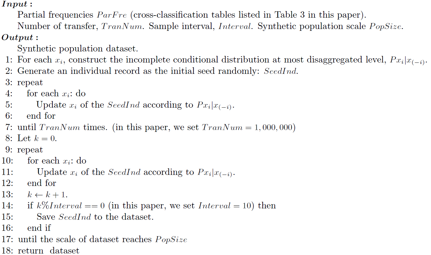
Markov Chain Monte Carlo (MCMC) simulation is a stochastic sampling technique to estimate overall distribution when the actual joint distribution is hard to access. Its theoretical foundation is that, if the stationary distribution of a Markov chain is a multivariate probability distribution, a sequence of observations can be approximately obtained through this chain. When applied to population synthesis, it firstly constructs a Markov chain with conditional transfer probabilities of each interested attribute (Farooq et al. 2013; Casati et al. 2015). Then samples are extracted from the chain at a particular interval, which is called Gibbs sampling. After the Gibbs sampler run for many iterations and reached a stationary state, this process is deemed as individual drawing from the actual population. Thus, the individual data set obtained can be directly used as synthetic population. Although the conditional transfer probabilities may be calculated from disaggregate sample, it is not essentially to do so. Actually, the conditional transfer probabilities are usually constructed by the input partial views from various data sources. Clearly, MCMC simulation is another sample-free synthetic method.
MCMC simulation is able to deal with both discrete and continuous attributes. It extends the scope of studied characteristics. However, when conditionals from different data sources are inconsistent, the Gibbs sampling may never reach a unique stationary state, which prevents the valid population drawing. In addition, the state transfer of Markov chain during discrete sampling may take an expensive time cost. As an emerging approach, this method needs further test and validation.
Population Synthesis Based on Joint Distribution Inference
As indicated in the previous section, IPFSR treats the association of disaggregate sample as that of target population, while CO does not preserve the complete association. Both of them ignore sample deviation and thus the generated population will not contain the type of individuals not included in the samples. Sample free fitting directly operates on individuals which seems computationally expensive. When generating a large scale population, MCMC simulation firstly constructs an individual pool to represent joint distribution, and then directly draws the synthetic population from the pool. When the combinations of variables are complicated, however, the pool will expand quickly in order to cover each potential type of individual. In this case, it will cost much time to conduct discrete sampling. Consequently, it is better to develop a new efficient synthetic method with the following highlights:
- Infer the joint distribution of target population directly. This could avoid redundant operations on individuals when adjusting each attribute.
- Use marginals and partial joint distributions as much as possible. It is able to maximize the utility of overall target population information and minimize sample deviations.
- Not necessarily require disaggregate samples. This enables our approach more applicable to general cases even if samples are not available.
- Should have a solid statistical and mathematical basis.
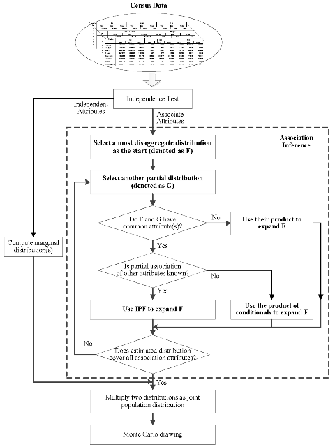
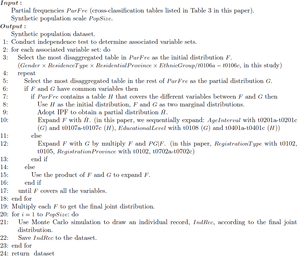
Starting from these objectives, our new method is composed of two steps: independence test and association inference. Figure 1 shows the main steps of the method, in which the association inference is most crucial.
Independence test
Independence test aims to validate whether two variables are independent of each other. According to probability theory, two random variables, X and Y, are called independent if and only if
| $$F(x,y)=F_{X}(x)\cdot F_{Y}(y),\ \forall x,y\in \mathbb{D}\notag$$ |
| $$f(x,y)=f_{X}(x)\cdot f_{Y}(y),\ \forall x,y\in \mathbb{D}\notag$$ |
| $$f(x_i,x_j)=f_{X_i}(x_i)\cdot f_{X_j}(x_j)\notag$$ |
| $$f(x_i,x_j)\ne f_{X_i}(x_i)\cdot f_{X_j}(x_j)\notag$$ |
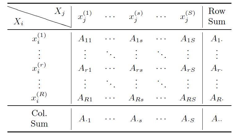
| $$\chi^{2}=\sum_{r=1}^{R}{\sum_{s=1}^{S}{\frac{(A_{rs}-\frac{A_{rs}}{A_{r\cdot}}\cdot \frac{A_{rs}}{A_{\cdot S}}\cdot A_{\cdot\cdot})^2}{\frac{A_{rs}}{A_{r\cdot}}\cdot \frac{A_{rs}}{A_{\cdot S}}\cdot A_{\cdot\cdot}}}} =\sum_{r=1}^{R}{\sum_{s=1}^{S}{\frac{(A_{r\cdot}\cdot A_{\cdot s}-A_{rs}\cdot A_{\cdot\cdot})^2}{A_{r\cdot}\cdot A_{\cdot s}\cdot A_{\cdot\cdot}}}}$$ |
If the studied attributes are partitioned into two sets and validated that \(\forall X_i\in\{X_1, X_2, \cdots, X_m\}\) is independent with \(\forall X_j\in\{X_{(m+1)}, X_{(m+2)}, \cdots, X_n\}\), the joint distribution can be denoted as
| $$f(x_1, \cdots, x_n)=f(x_1, \cdots, x_m)\cdot f(x_{m+1}, \cdots, x_n)\notag$$ |
| $$f(x_1, \cdots, x_n)=f_{X_i}(x_i)\cdot f(x_1, \cdots, x_{i-1}, x_{i+1}, \cdots, x_n)$$ |
 |
Association inference
Without loss of generality, assume the last \((n-m)\) attributes are independent, and rewrite Equation 2 as
| $$f(x_1, \cdots, x_n)=f(x_1, \cdots, x_m)\cdot f_{X_{m+1}}(x_{m+1})\cdot f_{X_{m+2}}(x_{m+2})\cdots f_{X_{n}}(x_{n})\notag$$ |
Suppose the start distribution is \(f(x_1, x_2)\). Consider another distribution \( f(x_1, x_3)\) where \(x_1\) is the common variable. Our objective is to estimate \(f(x_1, x_2, x_3)\). In theory, this contains infinite solutions without any further information. Thus, the basic idea is to construct one particular joint distribution that conforms to both of the partial views. The problem is categorized into two cases.
- \(f(x_2, x_3)\) is known. Then
where \(f_{X_1}(x_1)\) can be easily calculated from \(f(x_1, x_2)\) or \(f(x_1, x_3)\). Since \(x_2\) and \(x_3\) are not independent, their associations should be estimated. This task could be completed via IPF procedure. The Contingency Table involves two variables, \((x_2, x_3)\), and its initial seed is set according to \(f(x_2, x_3)\). For each given \(x_1\), IPF procedure is conducted and the corresponding marginals are computed as follows:$$ f(x_1, x_2, x_3)=f_{X_1}(x_1)\cdot f(x_2, x_3\mid x_1)$$ (3)
The result that IPF yields is denoted as \(f'(x_2, x_3\) and its marginals will conform to the above two conditional distributions. That is$$ f(x_2\mid x_1)=\frac{f(x_1, x_2)}{f_{X_1}(x_1)},\ f(x_3\mid x_1)=\frac{f(x_1, x_3)}{f_{X_1}(x_1)}\notag $$
The joint distribution is estimated by$$\begin{aligned} f'_{X_2}(x_2)&=\sum_{x_3}{f'(x_2, x_3)}=f(x_2\mid x_1)\\ f'_{X_3}(x_3)&=\sum_{x_2}{f'(x_2, x_3)}=f(x_3\mid x_1)\notag \end{aligned}$$
Comparing Equation 3 and 4, it is easy to find that the conditional probability \(f(x_2, x_3\mid x_1)\) is approximated by \(f'(x_2, x_3)\). The reason for this operation is \(f'(x_2, x_3)\) not only retains the associations between \(x_2\) and \(x_3\) but also satisfies the marginal constraints. It should be noted that the input \(f(x_2, x_3)\) may be acquired from a more complicated partial distributions by summarizing other unconsidered dimensions. This is a more general case which will be discussed later in this section.$$ f(x_1, x_2, x_3)=f_{X_1}(x_1)\cdot f'(x_2, x_3) $$ (4) - \(f(x_2, x_3)\) is unknown. In this case, all of the distributions do not contain associations between \(x_2\) and \(x_3\). It prevents us from estimating their joint distribution. Thus, their associations can simply be treated as the product of their conditionals. That is
Clearly, operations of the two cases above have extended the joint distribution. When this extension repeats until all the interested variables are included, the ultimate distribution is inferred.$$ \begin{aligned} f(x_1, x_2, x_3)=f_{X_1}(x_1)\cdot f(x_2, x_3\mid x_1)=f_{X_1}(x_1)\cdot f(x_2\mid x_1)\cdot f(x_3\mid x_1)\notag \end{aligned}$$
Now let us move to a general case. Suppose the start distribution is \(f(x_1, \cdots, x_k, x_{(k+1)}, \cdots, x_{(k+s)})\). Consider another partial view \(f(x_1, \cdots, x_l, x_{(k+s+1)}, \cdots, x_{(k+m)})\) where subscripts \(\{1, \cdots, l\}\subseteq\{1, \cdots, k\}\). For convenience, let \(X'_{1\cdot k}=(x_1, \cdots, x_k)\) and \(X'_{1\cdot l}\subseteq X'_{1\cdot k}\). If the partial distribution \(f(X'_{(k+1)\cdot (k+s)}, X'_{(k+s+1)\cdot (k+m)})\) is known, then the IPF procedure is adopted to estimate the associations that conform to the conditional marginal, \(f(X'_{(k+1)\cdot (k+s)}\mid X'_{1\cdot l})\) and \(f(X'_{(k+s+1)\cdot (k+m)}\mid X'_{1\cdot l})\). In order to construct the consistent marginals, it is required to exclude the unconcerned dimensions by summarizing these variables. That is
| $$f(X'_{(k+1)\cdot (k+s)}\mid X'_{1\cdot l})=\frac{f(X'_{1\cdot l}, X'_{(k+1)\cdot(k+s)})}{f(X'_{1\cdot l})}\notag $$ |
| $$\begin{aligned} f(X'_{1\cdot l}, X'_{(k+1)\cdot(k+s)})=\sum_{x_i}{f(X'_{1\cdot k}, X'_{(k+1)\cdot(k+s)})}\ \ \forall x_i\in X'_{1\cdot k}\ and\ x_i\notin X'_{1\cdot l}\notag \end{aligned}$$ |
| $$\begin{aligned} f(X'_{1\cdot l})=\sum_{x_i}{\sum_{x_j}{f(X'_{1\cdot k}, X'_{(k+1)\cdot (k+s)})}}\ \ \forall x_i\in X'_{1\cdot k}\ and\ x_i\notin X'_{1\cdot l}, x_j\in X'_{(k+1)\cdot (k+s)}\notag \end{aligned}$$ |
| $$f(X'_{(k+s+1)\cdot(k+m)}\mid X'_{1\cdot l})=\frac{f(X'_{1\cdot l}, X'_{(k+s+1)\cdot(k+m)})}{f(X'_{1\cdot l})}\notag $$ |
| $$\begin{aligned} f(X'_{1\cdot k}, X'_{(k+1)\cdot(k+s)}, X'_{(k+s+1)\cdot(k+m)})=f(X'_{1\cdot k})\cdot f'(X'_{(k+1)\cdot(k+s)}, X'_{(k+s+1)\cdot(k+m)})\notag \end{aligned}$$ |
| $$\begin{aligned} f(X'_{1\cdot k}, X'_{(k+1)\cdot(k+s)}, X'_{(k+s+1)\cdot(k+m)})=f(X'_{1\cdot k}, X'_{(k+1)\cdot(k+s)})\cdot f(X'_{(k+s+1)\cdot(k+m)}\mid X'_{1\cdot l})\notag \end{aligned}$$ |
Similar to the 3-dimensional case, the partial views \(f(X'_{(k+1)\cdot(k+s)}, X'_{(k+s+1)\cdot(k+m)})\) which used as the initial seed of IPF may be calculated from other more complicated distributions or even from sample data if it is accessible. The convergence of multivariate IPF in a general case is proved in the following. The convergence of multivariate IPF in a general case is proved in Appendix A.
Data Source
Census, traffic survey, labor force survey, tax record from revenue agency, real estate cadaster etc. are all primary data sources of synthetic population generation, though some of them are rarely used in practice. Household registration information in China also provides a supplement of micro individual data. Among all of the data sources, census has attracted most concentrations since it reflects the status of target population directly. In most countries census is conducted periodically, ranging from every 5 years (e.g, Canada) to every 10 years (e.g, U.S., Switzerland, China, etc.). The ultimate data officially published by Bureau of Statistics and other corresponding ministries are generally in two forms: sample of individuals and cross-classification table. As mentioned before, the disaggregate sample is usually used as a seed whereas the cross-classification tables are the basis of conditionals and marginals. The Public Use Microdata Samples (PUMS) in the U.S. and the Sample of Anonymized Records (SAR) in the UK are representatives of disaggregate samples, while typical aggregate tables include the Summary Files (SF), Standard Type File 3A (STF-3A) in the U.S. and the Small Area Statistics (SAS) in the UK. This paper mainly focuses on the population data available in China.
| Attributes | Number of Levels | Levels |
| Gender | 2 | Male, Female |
| Age Interval | 21 | 0-4, 5-9, ..., 95-99, 100 and above |
| Ethnic Group | 58 | Han, MengGu, Hui, ... |
| Residential Province | 31 | Beijing, Tianjin, ... |
| Educational Level | 10 | Infant, Not Educated, Literacy Class, Primary Sch.,Junior Mid. Sch., Senior Mid. Sch., Polytechnical Sch.,College, University, Graduate. |
| Residence Type | 3 | City, Town, Rural |
| Registration Province | 32 | Beijing, Tianjin, ..., Not Reg. |
| Registration Type | 2 | Agricultural, Non-agricultural |
Cross-classification table
Like many other countries, China conducts its national census for entire population every 10 years. Be-tween two adjacent censuses, a 1% population sample survey is conducted. In this paper, only the national census is considered. The most recent two censuses are in 2000 and 2010. The whole target populations are investigated through questionnaire under guidance of census takers. Two kinds of questionnaires are applied in the census. One is called the Short Table which involves several basic characteristics, whereas the other is the Long Table which not only contains all the content of the short one but also includes additional detailed features like migration pattern, educational level, economic status, marriage and family, procreation, housing condition, etc.. The Long Table is filled by individuals stochastically selected in advance (about 9.5% according to the official sampling rule), while the Short Table is completed by the rest. Results from these two kinds of questionnaires are the original individual records. They are usually confidential and will be further summarized over a few variables to get marginal frequencies. For instance, if the original records concern about (Gender x Residential Province x Age x Educational Level), the processed marginal frequencies may contain partial attributes like (Gender x Residential Province) or Educational Level. This operation is referred to as the data aggregation. Some but not all marginal frequencies are published on the website of National Bureau of Statistics (NBS) in the form of cross-classification tables (NBS 2000a, 2010). Appendix B gives three examples of them. This sort of data for public use is the fundamental information for population synthesis. Though these tables have not revealed the complete joint distribution of the whole attributes, they present its partial views in various dimensions.
In our study, we use the data of year 2000 to generate a synthetic population. The overall cross-classification tables concern a number of characteristics including population scale, gender, residential province, ethnic group, age, educational level, household scale and structure, dead people information, migration, housing condition, etc.. According to the census evaluation, about 1.81% of population is omitted in the survey[1]. It may slightly change the joint distribution. In addition, the census result does not contain information of military forces and organizations which are around 2,500,000 people. These two groups of people are also ignored in the synthetic process. In other words, our target population is those investigated in the overall data set. Since the objective of our study is to generate nationwide synthetic population, and the overall cross-classification tables cannot provide detailed attributes as the sample and Long Table do, we concentrate on the basic individual attributes shown in Table 2 (Where city refers to the municipality with the population density over 1500/km2. Town, outside the city, refers to the borough where the town government locates. Rural refers to the area other than city and town.). The corresponding partial distributions given by cross-classification tables are listed in Table 3. Note that the Table Codes are the ones used by the NBS.
| No. | Distributions | Table Codes |
| 1. | Gender x Residence Type x Residential Province | t0101a-t0101c |
| 2. | Gender x Residential x Province x Registration Type | t0102, t0105 |
| 3. | Gender x Residence Type x Residential Province x Ethnic Group | t0106a-t0106c |
| 4. | Gender x Residence Type x Residential Province x Age Interval | t0107a-t0107c |
| 5. | Gender x Residential Province x Educational Level | t0108 |
| 6. | Gender x Residence Type x Age Interval x Ethnic Group | t0201a-t0201c |
| 7. | Gender x Educational Level x Ethnic Group | t0202 |
| 8. | Gender x Residence Type x Age Interval x Educational Level | t0401a-t0401c |
| 9. | Residence Type x Residential Province x Registration Province | t0701a-t0701c t0702a-t0702c |
Sample
While total statistical characteristics can be easily acquired, original results directly from questionnaire are strictly protected by the government. Nevertheless, a small proportion of sample of the year 2000 have been collected. The data set includes 1,180,111 records, which accounts for 0.95% of the total population. These records all come from the Long Table, each of which gives detail information of a particular individual. The attributes provided by the sample can be categorized into two types. One is the basic household information such as household type (family or corporate), number of members, housing area, number of rooms, etc. while the other is the personal detailed attributes that involve employment status, occupation, marital status, number of children, etc.. Individual attributes contained in sample and the Long table are illustrated in Appendix C. Individual attributes contained in the sample and the Long Table can be referred to the website (NBS 2000b).
Long table
In contrast with the Short Table, the Long Table includes additional details, which reflects the structure and composition of target population much more concretely. People surveyed by this type of table are stochastically determined by NBS and each provincial government. Their scale accounts for 9.5% of total population. Their statistical results, in the form of cross-classification tables, can be also accessed from the official website. Since there is not any other data in this study, these tabulations are treated as our criterion to evaluate each synthetic population. The indicator adopted in our evaluation is the modified overall Relative Sum of Squared Z-scores (RSSZm) (Huang & Williamson 2001). For a given similar scaled subset of population being compared to the corresponding tabulations of the Long Table, that is:
| $$RSSZm=\sum_{k}{\sum_{i}{F_{ki}(O_{ki}-E_{ki})^2}}\notag $$ |
| $$\begin{split} F_{ki}=\left\{ \begin{array}{ll} \big(C_kO_{ki}\big(1-\frac{O_{ki}}{N_k}\big)\big)^{-1}, & if\ O_{ki}\ne0;\\ \frac{1}{C_k}, & if\ O_{ki}=0.\\ \end{array} \right. \notag \\ \end{split}$$ |
- \(O_{ki}\) is the generated count for the \(i\)-th cell of the \(k\)-th tabulation;
- \(E_{ki}\) is the given (known) count for the \(i\)-th cell of the \(k\)-th tabulation;
- \(N_k\) is the total count of tabulation \(k\);
- \(C_k\) is the 5\% \(\chi^2\) critical value for tabulation \(k\) (where degrees of freedom are treated as \(n-1\) for a table with \(n\) cells).
Details of the attributes in the Long Table are identical to the sample. It should be pointed out that the statistical results from the Long Table have not provided us information about Registration Province and Registration Type. Thus, our evaluation is only established on the rest of 6 characteristics.
Results
The five methods, IPFSR, CO, SFF, MCMC and the proposed method (referred as JDI), are used to generate a synthetic population of China. This section presents the results and gives an analysis about each synthetic population. Before showing the evaluation of generated synthetic populations, independence test results are presented according to Equation 1. Table 4 shows Chi-square values between every two attributes. These results all come from cross-classification tables of the total population. Note that the first line in each box is the Chi-square value whose magnitude is 104, and the two items in the second line of each box are degree of freedom and \(p\)-value (significance level \(\alpha=0.1\) respectively. As can be seen, no attribute is independent from others. This causes us to infer associations among all variables.
| Gender | Age Inter. | Ethnic group | Res. Prov. | Edu. Level | Res. Type | |
| Age Inter. | 179.11 20/28.41 | - | ||||
| Ethnic Group | 3.59 57/71.04 | 533.61 1140/1078.88 | - | |||
| Res. Type | 18.54 30/40.26 | 2677.44 600/644.8 | 281145.47 281145.47 | - | ||
| Edu. Level | 3315.31 9/14.68 | 5897.37 96/114.13 | 2958.93 513/554 | 7309.52 270/299 | - | |
| Res. Type | 1.79 2/4.61 | 1436.21 40/51.81 | 1763.42 114/133.73 | 11878.82 60/74.4 | 18372.58 18/25.99 | - |
| Reg. Prov. | 54.45 31/41.42 | - | - | 3493450.9 930/984.8 | - | 604.79 60/74.4 |
| Reg. Type | 31.76 2/4.61 | - | - | 7257.08 60/74.4 | - | - |
Note that our proposed JDI method is a sample-free method, and aims at providing a more efficient way than the two existing sample-free methods for a large scale population synthesis. Thus besides comparing the different methods from the accuracy point of view, their computational cost (in terms of execution time) are also measured and compared. Our goal is to show that the new method can generate synthetic population with the same level of accuracy as the existing sample-free methods, but is much more computational efficient. Meanwhile, since our data includes samples, it is possible to generate synthetic population using the sample-based methods. The results from these sample-based methods are also presented, and comparing all these different methods (sample-based and sample-free) for a large scale population synthesis is also considered as one of the contributions of this paper.
In our study, all the tables listed in Table 3 are used as the inputs of the sample-free methods. The scale of synthetic population generated by the five methods is 1,242,612,226 (total Chinese population). According to the Long Table scale, 9.5% of the synthetic populations are stochastically extracted for quantitative evaluations. In order to reduce the impacts of randomness, each experiment is conducted 5 times and averaged to obtain the final results in this section. The evaluations are composed of two parts. Firstly, since Registration Type and Registration Province are missing in the statistical results of the Long Table, marginal consistency of the rest 6 attributes (Gender, Age Interval, Ethnic Group, Residential Province, Educational Level, Residence Type) are investigated. Secondly, partial joint distributions of specific attributes are also given in the Long Table results. They can be used to calculate RSSZm value in a more detailed way. The RSSZm indicator has been introduced in previous section, and the partial joint distributions adopted as our reference criterion are shown in Table 5.
| No. | Distributions | Table Codes |
| 1. | Gender x Residence Type x Residential Province | l0101a-l0101c |
| 2. | Gender x Residence Type x Age Interval | l0102a-l0102c |
| 3. | Gender x Ethnic Group | l0201, l0203 |
| 4. | Gender x Residence Type x Educational Level | l0301a-l0301c |
Marginal consistency
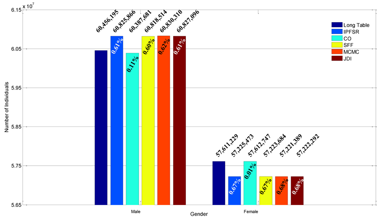
The population sizes derived from Long Table and five methods are 118,067,424 (Long Table), 118,051,339 (IPFSR), 118,000,428 (CO), 118,042,198 (SFF), 118,051,699 (MCMC) and 118,049,388 (JDI), respectively. The minor difference stems from the stochastic sampling according to 9.5%. Figure 2 gives the statistical result of gender marginal. As can be seen, all errors are below 400,000 which accounts for 0.66% (male) and 0.69% (female). The sample-based method CO performs the best with its error 68,514 (male) and 1,518 (female).
The age interval marginal comparison is shown in Figure 3. Similarly, the two sample-based methods result in more accurate match with the Long Table data, while the three sample-free ones have brought minor deviations. The proposed JDI method shows a similar performance with other sample-free methods. The trend of lines also indicates two “baby booms” in Chinese history.
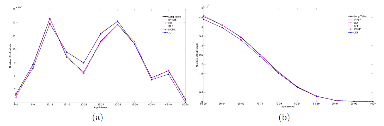
Figure 4 gives comparison of ethnic groups, among which the major—Han group—accounts for over 90% and is shown by the line with 1.14%, 0.37%, 0.94%, 0.80%, 1.16% relative errors. Individual numbers of other 55 minor ethnic groups are summarized and shown by the bar figure. Their relative errors are all below 5%. Unrecognized ethnic group and foreigners are calculated in Table 6. It is important to note that IPFSR and CO do not contain individuals from the unrecognized group. The reason of this phenomenon is our input sample does not include this type of person. This “zero element” problem cannot be solved by the sample-based methods. Thus, under this condition, the limitations of the sample-based methods are apparent.
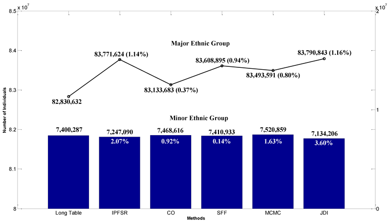
| Unrecognized Ethnic Group | Foreigner | |
| Long Table | 47,523 | 110 |
| IPFSR | 0 | 65 |
| CO | 0 | 51,114 |
| SFF | 47,786 | 68 |
| MCMC | 51,307 | 79 |
| JDI | 33,191 | 27 |
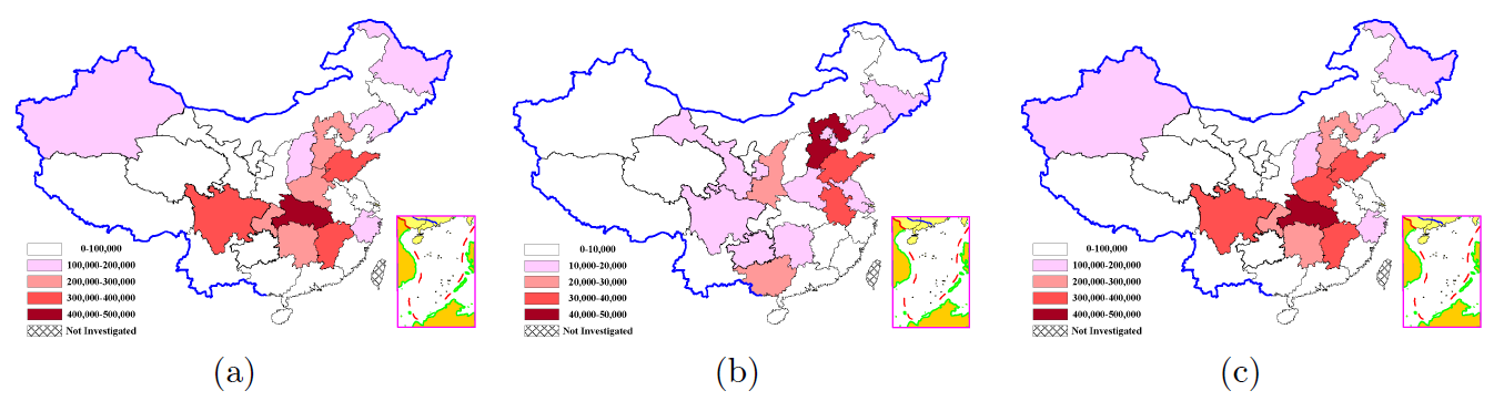
The populations for the 31 provinces of China are compared in Figure 5. Absolute deviations between the sampled synthetic populations and the Long Table data are represented by different color in the map. Note the numerical range represented by each type of color in subfigure 5(b) is different from others. As can be seen, the CO result always outperforms others. This is due to its generation mechanism. Different from others, CO partitions the whole population into several parts and generates it one by one in its synthetic process. This accurately controls synthetic population in smaller scales. Thus, CO brings the best results. The figure also shows the rest of the methods have similar errors.
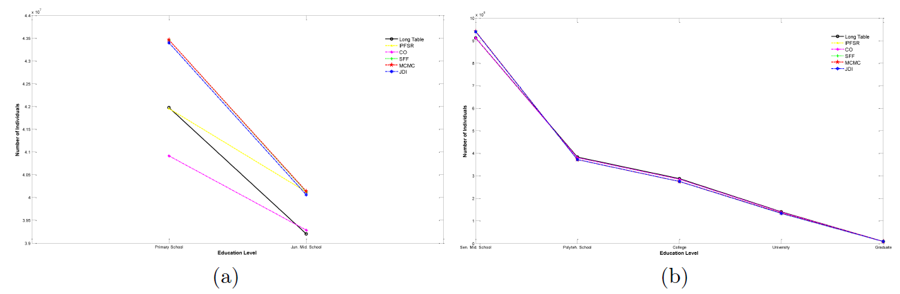
For the educational level, the census only investigates individuals over 6 years old. Thus, our evaluation also focuses on these populations. The Long Table and five synthetic results are drawn in Figure 6. As can be seen, each educated group percentage of these methods is nearly the same. Quantitatively, the average relative errors are 3.20% (IPFSR), 1.49% (CO), 3.69% (SFF), 3.68% (MCMC) and 3.68% (JDI). It seems that the sample can elevate the accuracy of this marginal indicator.
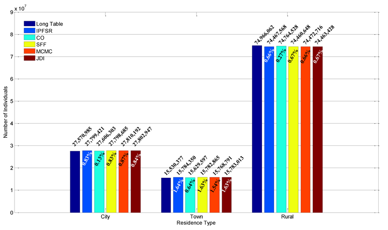
The last marginal attribute is residence type, the results of which are presented in Figure 7. From the figure, about two thirds of the people are living in rural areas in 2000, and each residence type has a similar percentage. It shows the five methods all have good results when measured by this marginal.
The marginal mean absolute errors (MAE) and root mean squared errors (RMSE) are computed Table 7. Generally, the CO method has better performance than the others. And all of them show a relative worse result in ethnic group, especially CO. The large MAE and RMSE deviations are also caused by the deficiency of specific type of individuals in sample. The three sample-free methods have a similar accuracy in marginal consistencies.
| Gender | Age Inter. | Ethnic Group | Res. Prov. | Edu. Level | Res. Type | |||||||
| MAE | RMSE | MAE | RMSE | MAE | RMSE | MAE | RMSE | MAE | RMSE | MAE | RMSE | |
| IPFSR | 0.64 | 377,799 | 3.69 | 268,701 | 12.68 | 123,982 | 3.25 | 178,383 | 3.20 | 372,811 | 1.04 | 348,894 |
| CO | 0.06 | 48,459 | 2.34 | 90,971 | 820.03 | 40,975 | 0.43 | 17,239 | 1.49 | 402,998 | 0.35 | 131,286 |
| SFF | 0.64 | 375,144 | 3.78 | 268,892 | 6.29 | 102,547 | 3.24 | 177,453 | 3.69 | 671,501 | 1.04 | 351,682 |
| MCMC | 0.65 | 382,058 | 3.90 | 269,218 | 7.52 | 87,432 | 3.29 | 178,076 | 3.68 | 676,170 | 1.02 | 345,182 |
| JDI | 0.64 | 380,026 | 12.88 | 266,461 | 27.18 | 126,592 | 3.26 | 178,052 | 3.68 | 639,449 | 1.05 | 351,318 |
Partial joint distribution consistency
Table 8 gives the RSSZm results which have been introduced before. The main deviation comes from Gender x Ethnic Group distribution, and the three sample-free methods generated better population databases than the sample-based ones. The reason for this phenomenon is that the sample-free methods treat associations among individual attributes reflected by partial joint distributions as their inputs, and these associations are derived from the whole target population. Thus, the sample-free methods are able to directly manipulate total population associations rather than the sample which most likely carries deviation in sampling process. The results also show SFF and JDI have relatively smaller RSSZm values.
| Gender x Res. Type x Res. Prov. (l0101a-l0101c) | Gender x Res. Type x Res. Prov. (l0102a-l0102c) | Gender x Ethnic Group (l0201,l0203) | Gender x Res. Type x Edu. Level (l0301a-l0301c) | Total | |
| IPFSR | 1,053 | 1,358 | 8,020,954 | 1,055 | 8,024,420 |
| CO | 85 | 275 | 8,021,125 | 683 | 8,022,168 |
| SFF | 1,097 | 1,297 | 313 | 2,162 | 4,869 |
| MCMC | 1,098 | 8,962 | 310 | 245,325 | 255,695 |
| JDI | 1,101 | 1,312 | 3,446 | 2,109 | 7,968 |
MAE and RMSE of partial joint distributions are also calculated in Table 9. It can be seen that CO and MCMC get the largest MAE and RMSE (most come from Gender Ethnic Group and Gender x Residence Type x Educational Level distributions), and IPFSR and SFF perform the best. Among the three sample-free methods, SFF is a little better than JDI and they both outperform MCMC.
In summary, the population databases synthesized by the sample-based methods, especially CO, have better performances on marginal indicators, while the sample-free methods generated populations that match partial joint distributions more precisely. The SFF and JDI methods have similar accuracy among the sample-free methods, both of which are a little higher than MCMC.
| Gender x Res Type x Res. Prov. (l0101a-l0101c) | Gender x Res Type x Res. Prov. (l0102a-l0102c) | Gender x Ethnic Group (l0201,l0203) | Gender x Res Type x Edu. Level (l0301a-l0301c) | Total | ||||||
| MAE | RMSE | MAE | RMSE | MAE | RMSE | MAE | RMSE | MAE | RMSE | |
| IPFSR | 3.89 | 38,867 | 6.99 | 57,996 | 23.33 | 72,740 | 5.01 | 76,779 | 9.62 | 57,725 |
| CO | 1.72 | 7,384 | 5.95 | 21,297 | 1006.79 | 20,678 | 4.23 | 95,046 | 251.14 | 32,496 |
| SFF | 3.43 | 42,891 | 4.17 | 55,002 | 6.95 | 72,148 | 6.52 | 128,619 | 4.77 | 65,590 |
| MCMC | 3.47 | 42,982 | 9.74 | 150,972 | 8.30 | 68,748 | 321.04 | 805,836 | 34.72 | 256,976 |
| JDI | 3.43 | 43,077 | 24.58 | 54,881 | 28.99 | 81,885 | 5.96 | 122,407 | 15.64 | 67,347 |
Computational performance
Synthesizing nationwide population database of China is a large project. Consequently, computational performance is another important metric that should not be ignored. To achieve meaningful comparison from the computational cost point of view, we implemented all the five methods in the same programming environment and run the methods on the same computer. More specifically, we implemented the five methods in C# .net framework environment and run the programs on an Intel Core i7-4790 CPU with 8 GB RAM. The execution time is divided into two parts: distribution computing (if there is) and population realization. The averaged results of the five methods are listed in Table 10.
| Method | Distribution Computing | Population Realization | Environment |
| IPFSR | 08 Hour(s) 01 Min(s) | 2 Day(s) 08 Hour(s) 18 Min(s) | Software: C# .net framework |
| CO | - | 8 Day(s) 21 Hour(s) 50 Min(s) | OS: Windows 7 (x64) |
| SFF | - | 6 Day(s) 16 Hour(s) 41 Min(s) | CPU: Intel Core i7-4790 |
| MCMC | 6 Day(s) 21 Hour(s) 52 Min(s) | 10 Hour(s) 57 Min(s) | (8 cores, 3.6GHz) |
| JDI | 03 Hour(s) 47 Min(s) | 2 Day(s) 09 Hour(s) 38 Min(s) | RAM: 8 GB |
It is clear that among the five methods, our proposed method JDI costs the least amount of execution time. Although CO has relatively accurate results as aforementioned, it is also the most computationally expensive one. During its computation, the total target population is partitioned into 100 parts and generated one by one for its convergence. The MCMC method has the second worst performance when comparing with others. The main reason is that MCMC builds its joint distribution by constructing an individual pool via discrete sampling from the Markov Chain. According to the MCMC theory, after Gibbs sampler achieved its stationary state, successive sampling should be prevented in order to avoid any correlations between two adjacently generated individuals. To this end, synthetic individuals are usually drawn at a particular interval rather than from each chain update. In our study, this interval is set to be 10 iterations. The size of the individual pool is set to be 50 million. Therefore, it costs a large amount of computation. The SFF method is a little better than MCMC. This is mainly due to frequent updates on the individual pool, which causes substantial I/O operations on database. In contrast with RAM access, database manipulation seems much slower. IPFSR is much faster than the above three. It directly fits the joint distribution of the population and draws individuals. It directly fits the joint distribution of the population and draws individuals at a time. This approach, however, usually suffers from rapid growth in calculation as the investigated attributes increase. In our scenario, the theoretical number of attribute combinations is about \(1.4\times 10^8\) (including some zero cells in joint distribution). Fitting these combinations is, undoubtedly, much complicated and soars its computational time. On the other hand, Monte Carlo realization of individual records needs conditional probability rather than the joint distribution itself. Thus, in contrast with IPFSR, our JDI method directly calculates conditional distributions after each variable expansion. To a certain extent, this reduces the computational complexity since the attribute combinations are much fewer at the beginning of its computation. It should be pointed out that the access to database in all the five methods uses a single-threaded pattern. Multi-threaded techniques are expected to accelerate the programs but more attention needs to be paid to the data synchronization.
A small area test
In order to further validate our proposed method, numerical experiments for a smaller area are also conducted. We choose the population of Qingdao—a coastal city of middle size—to be our target population. The total scale of the target population is about 7.5 million, much smaller than that of the whole nation. Similarly, our available data source contains the regional overall cross-classification tables and the relevant Long Tables. But the attributes and their input distributions revealed from this regional data are not as sufficient as those of the nationwide. Specifically, the Long Tables only give the Gender District frequencies of individuals whose age are beyond 15. Table 11 shows the attributes considered. The distributions of the Short and Long Tables are listed in Table 12. Since the disaggregate sample cannot distinguish among different districts, two sample-based methods are not able to generate synthetic population at this granularity. Here we only focus on the sample-free methods.
| Attributes | Number of Levels | Levels |
| Gender | 2 | Male, Female |
| ShiNan, ShiBei, SiFang, HuangDao, | ||
| District | 12 | LaoShan, LiCang, ChengYang, JiaoZhou, |
| JiMo, PingDu, JiaoNan, LaiXi | ||
| Residence Type | 2 | Urban, Rural |
| Infant, Not Educated, Liter. Class, Pri. Sch., | ||
| Educational Level | 10 | Jun. Mid. Sch., Sen. Mid. Sch., Polyteh. Sch., |
| College, University, Graduate | ||
| Age Interval | 18 | 0-4, 5-9,… , 85 and above |
| No. | Short Table (Inputs) | No. | Long Table (Evaluation Criteria) |
| 1 | District x Residence Type | 1 | Gender x District (for Age ≥ 15) |
| 2 | Gender x District x Age Interval | ||
| 3 | Gender x District x Educational Level |
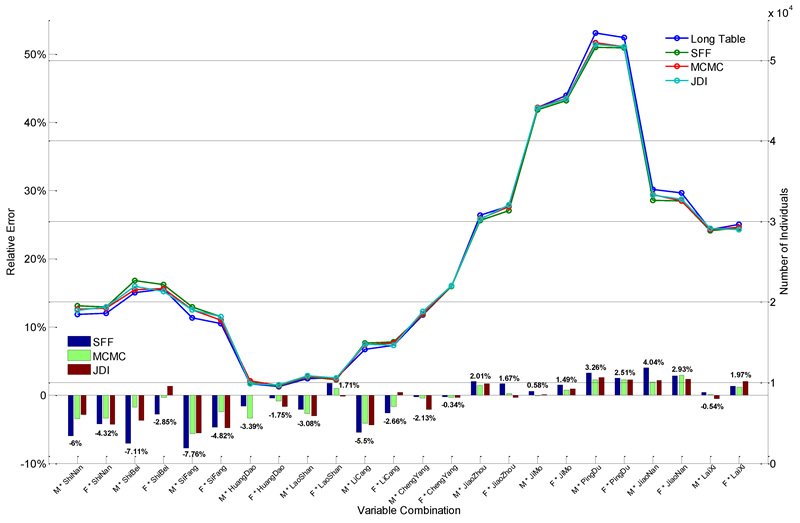
Like the nationwide scenario, the experiment is repeated 5 times and a small proportion of each result is stochastically sampled according to the Long Table population scale. The sampled populations are evaluated respectively, and the averaged final result is shown in Figure 8. As can be seen, the largest error is -7.76% and most of them are below 5%. The three RSSZm values are 18.6998(SFF), 8.1140(MCMC), and 10.2088(JDI). It indicates that the latter two perform much better in general. As RSSZm measures the deviation between real and synthetic data, the results also manifest the proposed algorithm is robust at the district level.
Conclusions and Discussions
The paper reviewed the existing four major population synthesis methods—synthetic reconstruction, combinatory optimization, sample free fitting, and MCMC simulation—and then presented a new sample-free method based on joint distribution inference. These methods are applied to synthesize a nationwide population database of China by using its cross-classification tables and a 0.95% sample from census. The methods are evaluated and compared quantitatively by measuring marginal and partial joint distribution consistencies and computational cost. Our results indicated that the two sample-based methods, IPFSR and CO, show a better performance on marginal indicators, whereas the sample-free ones especially SFF and JDI give a relatively small error on partial distributions. Moreover, the proposed JDI gets a better computational performance among the five methods.
Cross-classification tables, sample and long tables used in this paper are all from the census data, where data inconsistency does not arise explicitly. As explained in Section 4, however, various data sources can be used as the inputs to generate synthetic population. Adopting multiple input data sources may probably suffer from the data inconsistency, which will hamper the convergence of the computational process. Our proposed JDI method can also cope with such problem to some extent. After an independence test, the joint distribution inference of remaining associated variables also consists of distribution initialization and variable expansion. Similarly, we can represent the constraints from two data sources as a group of marginal or partial distributions. Without loss of generality, assume that \(u(x_1,\cdots,x_m)\) and \(v(x_1,\cdots,x_n) (m\leq n)\) are the most disaggregate ones from the two groups respectively. There are several mechanisms that determine the initial distribution. For example, a confidence evaluation of the two data sources can be conducted in advance and the more confidential one is used as the start point. Or alternatively, if \(m=n\) (the variables in \(v\) but \(u\) can be folded to satisfy this assumption), the following averages can be used as the initial distribution:
| $$f(x_1,\cdots,x_m)=\alpha\cdot u(x_1,\cdots,x_m)+\beta\cdot v(x_1,\cdots,x_n)\notag$$ |
As shown in Section 2 and Appendix D, CO usually partitions the target population into a set of smaller identical parts, and generates each of them as the final result. Accordingly, the fitness criterion for each small part is proportionally scaled down by the overall statistical marginals. Such operation will not bring bias to the CO method. Here we give a brief analysis. Let \(Pop_N\) be the total target population (unknown), \(S_N\) be the overall statistical marginals used as the criterion, \(k\) be the partition number (integer). Then for the \(i\)-th part, we have \(Pop_i=Pop_N/k \) and \(S_i=S_N/k\). If we initially set a common convergence relative error \(\varepsilon_i=\varepsilon\) for every part, the following equation holds when the iteration of part \(i\) stops:
| $$\varepsilon_i=\varepsilon=\frac{|Pop_i-S_i|}{S_i}=\frac{|Pop_N/k-S_N/k|}{S_N/k}=\frac{|Pop_N-S_N|}{S_N}=\varepsilon_N\notag $$ |
For sample-based methods, the bias of input sample will be retained in the final synthetic population inevitably. This can be avoided to some extent by sample-free techniques which treat the total population features as their start points. However, sample-free methods cannot merit the advantage of disaggregate sample—associations among all the investigated attributes. Like others, the JDI proposed in this paper uses partial joint distributions instead. But for those variables whose association with others cannot be estimated from known partial views (for instance, only one marginal distribution involves a particular attribute, and the associations between this attribute and other variables cannot be well estimated), sample is usually a direct and beneficial supplement.
Several possible directions can be extended in the future research. To name a few, two of them are put forward here. Firstly, it is obvious that the census data play a much important role in population synthesis. It is even more important when using sample-free methods. However, the available input data with desired quality are not always possible, since the census results may contain errors to some extent in their survey and statistical process. Therefore, other sorts of data, such as family and household, need to be introduced to reduce that kind of errors. Related work has been conducting by many scholars (see, e.g. Anderson et al. 2014 and Casati et al. 2015). Yet how to solve the conflict between individual and household level constraints requires further study. Secondly, large scale population synthesis and the subsequent micro-simulation are much time consuming and computational expensive. This low efficiency usually leads to the loss of effectiveness in the computer-aided decision making. Two possible approaches may contribute to the solution of this problem. One is expanding the computational resources by introducing parallel and distributed computing. It involves massive data and its synchronization in a distributed pattern, and thus deserves carefully researched. The other concerns the optimization of algorithms and simulation models. Building an extremely detailed agent model in the subsequent micro-simulation is unfeasible and unnecessary. Thus, the principle and framework of establishing appropriate agent behavioral models under available computational resources also require to be carefully considered.
Acknowledgements
This research was supported by National Natural Science Foundation of China (No. 61603381, 71472174, 61533019, 71232006), and Award from Department of Energy, USA (No. 4000152851).Notes
- In order to evaluate the quality of the 5th census, the NBS conducted a post-enumeration survey for quality check. 602 nationwide census blocks were stochastically determined by the Stratified Sampling, and were investigated two weeks after the census. Results of these blocks from the survey and the census were compared to calculate deviations. The missing rate for the total recorded population is estimated from the weighted summary of the deviations.
Appendix
Appendix A: Convergence analysis
Since the IPF method proposed by Deming & Stephan (1940), its convergence has been extensively investigated (Fienberg 1970; Pretzel 1980; Ruschendorf 1995; Pukelsheim 2014). However, these related literatures have only considered 2-dimensional case. This subsection will give a proof for a general case. In order to illustrate the main thought, 3-dimensional case is firstly presented and then extended to a multivariate case.
Proposition 1 (3-dimensional case). Suppose the marginals of three positive real variables (X1; X2; X3) are f(x1), f(x2) and f(x3). The result of k-th iteration can be written as
| $$f^{(1)}(x_1, x_2, x_3)(k)=\frac{f(x_1, x_2, x_3)(k-1)}{\sum_{x_2, x_3}{f(x_1, x_2, x_3)(k-1)}}\cdot f(x_1)\ \ (x_1\ fitted)\\ $$ |
| $$f^{(2)}(x_1, x_2, x_3)(k)=\frac{f^{(1)}(x_1, x_2, x_3)(k)}{\sum_{x_1, x_3}{f^{(1)}(x_1, x_2, x_3)(k)}}\cdot f(x_2)\ \ (x_2\ fitted)\\ $$ |
| $$f^{(3)}(x_1, x_2, x_3)(k)=\frac{f^{(2)}(x_1, x_2, x_3)(k)}{\sum_{x_1, x_2}{f^{(2)}(x_1, x_2, x_3)(k)}}\cdot f(x_3)\ \ (x_3\ fitted)\notag $$ |
| $$f(x_1, x_2, x_3)(k)=f^{(3)}(x_1, x_2, x_3)(k)\notag $$ |
Define L1 error as
| $$L(k)=\sum_{x_1}{\Bigg|\sum_{x_2, x_3}{f(x_1, x_2, x_3)(k)}-f(x_1)\Bigg|}+\sum_{x_2}{\Bigg|\sum_{x_1, x_3}{f(x_1, x_2, x_3)(k)}-f(x_2)\Bigg|}+\sum_{x_3}{\Bigg|\sum_{x_1, x_2}{f(x_1, x_2, x_3)(k)}-f(x_3)\Bigg|}\notag$$ |
Then the L1 error monotonously decreases during its iteration.
Proof: When \(X_1\), \(X_2\) and \(X_3\) are fitted in turn during the \(k\)-th iteration, L1 errors are
| $$\begin{aligned}L^{(1)}(k)=&\sum_{x_2}{\Bigg|\sum_{x_1, x_3}{f^{(1)}(x_1, x_2, x_3)(k)}-f(x_2)\Bigg|}+\sum_{x_3}{\Bigg|\sum_{x_1, x_2}{f^{(1)}(x_1, x_2, x_3)(k)}-f(x_3)\Bigg|}\\ L^{(2)}(k)=&\sum_{x_1}{\Bigg|\sum_{x_2, x_3}{f^{(2)}(x_1, x_2, x_3)(k)}-f(x_1)\Bigg|}+\sum_{x_3}{\Bigg|\sum_{x_1, x_2}{f^{(2)}(x_1, x_2, x_3)(k)}-f(x_3)\Bigg|}\\ L^{(3)}(k)=&\sum_{x_1}{\Bigg|\sum_{x_2, x_3}{f^{(3)}(x_1, x_2, x_3)(k)}-f(x_1)\Bigg|}+\sum_{x_2}{\Bigg|\sum_{x_1, x_3}{f^{(3)}(x_1, x_2, x_3)(k)}-f(x_2)\Bigg|}\notag \end{aligned}$$ |
Similarly for the \((k + 1)\)-th iteration:
| $$\begin{aligned}L^{(1)}(k+1)=&\sum_{x_2}{\Bigg|\sum_{x_1, x_3}{f^{(1)}(x_1, x_2, x_3)(k+1)}-f(x_2)\Bigg|}+\sum_{x_3}{\Bigg|\sum_{x_1, x_2}{f^{(1)}(x_1, x_2, x_3)(k+1)}-f(x_3)\Bigg|}\\ L^{(2)}(k+1)=&\sum_{x_1}{\Bigg|\sum_{x_2, x_3}{f^{(2)}(x_1, x_2, x_3)(k+1)}-f(x_1)\Bigg|}+\sum_{x_3}{\Bigg|\sum_{x_1, x_2}{f^{(2)}(x_1, x_2, x_3)(k+1)}-f(x_3)\Bigg|}\\ L^{(3)}(k+1)=&\sum_{x_1}{\Bigg|\sum_{x_2, x_3}{f^{(3)}(x_1, x_2, x_3)(k+1)}-f(x_1)\Bigg|}+\sum_{x_2}{\Bigg|\sum_{x_1, x_3}{f^{(3)}(x_1, x_2, x_3)(k+1)}-f(x_2)\Bigg|}\notag \end{aligned}$$ |
| $$\begin{aligned}\sum_{x_2}{\Bigg|\sum_{x_1, x_3}{f^{(1)}(x_1, x_2, x_3)(k)}-f(x_2)\Bigg|}&=\sum_{x_2}{\Bigg|\sum_{x_1, x_3}{f^{(1)}(x_1, x_2, x_3)(k)}-\sum_{x_1, x_3}{f^{(2)}(x_1, x_2, x_3)(k)}\Bigg|}\\ & =\sum_{x_2}{\Bigg|\sum_{x_1, x_3}{\Big(f^{(1)}(x_1, x_2, x_3)(k)-f^{(2)}(x_1, x_2, x_3)(k)\Big)}\Bigg|} \end{aligned}$$ | (5) |
| $$f^{(2)}(x_1, x_2, x_3)(k)=\frac{f^{(1)}(x_1, x_2, x_3)(k)}{\rho(x_2)(k)}\notag$$ |
| $$\rho(x_2)(k)=\frac{\sum_{x_1, x_3}{f^{(1)}(x_1, x_2, x_3)(k)}}{f(x_2)}\notag$$ |
Clearly, \(\rho(x_2)(k)\) only depends on \(x_2\). Thus for a given \(x_2\), each \(f^{(1)}(x_1, x_2, x_3)(k)-f^{(2)}(x_1, x_2, x_3)(k)=(1-\frac{1}{\rho(x_2)(k)})\cdot f^{(1)}(x_1, x_2, x_3)(k)\) has the same sign, and Equation 5 can be written as
| $$\sum_{x_2}{\Bigg|\sum_{x_1, x_3}{\Big(f^{(1)}(x_1, x_2, x_3)(k)-f^{(2)}(x_1, x_2, x_3)(k)\Big)}\Bigg|}=\sum_{x_1, x_2,x_3}{\Bigg|f^{(2)}(x_1, x_2, x_3)(k)-f^{(1)}(x_1, x_2, x_3)(k)\Bigg|}$$ | (6) |
According to triangle inequality, it can be obtained immediately that
| $$\begin{aligned} \sum_{x_1, x_2, x_3}{\Bigg|f^{(2)}(x_1, x_2, x_3)(k)-f^{(1)}(x_1, x_2, x_3)(k)\Bigg|}&\geq\sum_{x_1}{\Bigg|\sum_{x_2, x_3}{\Big(f^{(2)}(x_1, x_2, x_3)(k)-f^{(1)}(x_1, x_2, x_3)(k)\Big)}\Bigg|}\\ &=\sum_{x_1}{\Bigg|\sum_{x_2, x_3}{f^{(2)}(x_1, x_2, x_3)(k)}-f(x_1)\Bigg|} \end{aligned}$$ | (7) |
On the other hand,
| $$\begin{aligned} \sum_{x_1}{\Bigg|\sum_{x_2, x_3}{f^{(2)}(x_1, x_2, x_3)(k)}-f(x_1)\Bigg|}=\sum_{x_1}{\Bigg|\sum_{x_2, x_3}{\Big(f^{(2)}(x_1, x_2, x_3)(k)-f^{(1)}(x_1, x_2, x_3)(k+1)\Big)}\Bigg|} \end{aligned}$$ | (8) |
| $$f^{(1)}(x_1, x_2, x_3)(k+1)=\frac{f^{(2)}(x_1, x_2, x_3)(k)}{\rho(x_3)(k)\cdot\rho(x_1)(k+1)}\notag $$ |
| $$\rho(x_3)(k)=\frac{\sum_{x_1, x_2}{f^{(2)}(x_1, x_2, x_3)(k)}}{f(x_3)}\notag $$ |
| $$\begin{aligned} \rho(x_1)(k+1)=\frac{\sum_{x_2, x_3}{f^{(3)}(x_1, x_2, x_3)(k)}}{f(x_1)}=\frac{1}{f(x_1)}\cdot\sum_{x_2, x_3}{\Bigg[\frac{f^{(2)}(x_1, x_2, x_3)(k)}{\sum_{x_1, x_2}{f^{(2)}(x_1, x_2, x_3)(k)}}\cdot f(x_3)\Bigg]}\notag \end{aligned} $$ |
Obviously, \(\sum_{x_1, x_2}{f^{(2)}(x_1, x_2, x_3)(k)}\) only depends on \(x_3\). Denote \(M^{(2)}(x_3)=\sum_{x_1, x_2}{f^{(2)}(x_1, x_2, x_3)(k)}\) for convenience. Thus
| $$\begin{aligned} \rho(x_1)(k+1)=\frac{1}{f(x_1)}\cdot\sum_{x_2, x_3}{\Bigg[\frac{f^{(2)}(x_1, x_2, x_3)(k)}{\sum_{x_1, x_2}{f^{(2)}(x_1, x_2, x_3)(k)}}\cdot f(x_3)\Bigg]}=\frac{1}{f(x_1)}\cdot\sum_{x_3}{\Bigg[\frac{f(x_3)}{M^{(2)}(x_3)}\cdot\Big(\sum_{x_2}{f^{(2)}(x_1, x_2, x_3)(k)}\Big)\Bigg]}\notag \end{aligned}$$ |
Again, \(\sum_{x_2}{f^{(2)}(x_1, x_2, x_3)(k)}\) only depends on \(x_1\) and \(x_3\). We denote it as \(N^{(2)}(x_1, x_3)=\sum_{x_2}{f^{(2)}(x_1, x_2, x_3)(k)}\) for convenience. Then
| $$\begin{aligned} \rho(x_1)(k+1)=\frac{1}{f(x_1)}\cdot\sum_{x_3}{\Bigg[\frac{f(x_3)}{M^{(2)}(x_3)}\cdot\Big(\sum_{x_2}{f^{(2)}(x_1, x_2, x_3)(k)}\Big)\Bigg]}=\frac{1}{f(x_1)}\cdot\sum_{x_3}{\Bigg(\frac{N^{(2)}(x_1, x_3)}{M^{(2)}(x_3)}\cdot f(x_3)\Bigg)}\notag \end{aligned}$$ |
As can be seen, \(\rho(x_1)(k+1)\) is not relevant to \(x_2\). Consequently, for any \(x_2\), each
| $$\begin{aligned} \sum_{x_3}{\bigg(f^{(2)}(x_1, x_2, x_3)(k)-f^{(1)}(x_1, x_2, x_3)(k+1)\bigg)}=\sum_{x_3}{\bigg(1-\frac{1}{\rho(x_3)(k)\cdot\rho(x_1)(k+1)}\bigg)f^{(2)}(x_1, x_2, x_3)(k)}\notag \end{aligned}$$ |
| $$\begin{aligned} \sum_{x_1}{\Bigg|\sum_{x_2, x_3}{\Big(f^{(2)}(x_1, x_2, x_3)(k)-f^{(1)}(x_1, x_2, x_3)(k+1)\Big)}\Bigg|}=\sum_{x_1, x_2}{\Bigg|\sum_{x_3}{\Big(f^{(2)}(x_1, x_2, x_3)(k)-f^{(1)}(x_1, x_2, x_3)(k+1)\Big)}\Bigg|}\notag \end{aligned}$$ |
Also, the triangle inequality leads to
| $$\begin{aligned} \sum_{x_1, x_2}{\Bigg|\sum_{x_3}{\Big(f^{(2)}(x_1, x_2, x_3)(k)-f^{(1)}(x_1, x_2, x_3)(k+1)\Big)}\Bigg|}&\geq\sum_{x_2}{\Bigg|\sum_{x_1, x_3}{\Big(f^{(1)}(x_1, x_2, x_3)(k+1)-f^{(2)}(x_1, x_2, x_3)(k)\Big)}\Bigg|}\\ &=\sum_{x_2}{\Bigg|\sum_{x_1, x_3}{f^{(1)}(x_1, x_2, x_3)(k+1)}-f(x_2)\Bigg|} \end{aligned}$$ | (9) |
From Equation 5 to Equation 9, there is
| $$\begin{aligned} \sum_{x_2}{\Bigg|\sum_{x_1, x_3}{f^{(1)}(x_1, x_2, x_3)(k)}-f(x_2)\Bigg|}\geq\sum_{x_2}{\Bigg|\sum_{x_1, x_3}{f^{(1)}(x_1, x_2, x_3)(k+1)}-f(x_2)\Bigg|}\notag \end{aligned}$$ |
| $$\begin{aligned} \sum_{x_3}{\Bigg|\sum_{x_1, x_2}{f^{(1)}(x_1, x_2, x_3)(k)}-f(x_3)\Bigg|}\geq\sum_{x_3}{\Bigg|\sum_{x_1, x_2}{f^{(1)}(x_1, x_2, x_3)(k+1)}-f(x_3)\Bigg|}\notag \end{aligned}$$ |
Therefore, \(L^{(1)}(k)\geq L^{(1)}(k+1)\). \(L^{(2)}(k)\) and \(L^{(3)}(k)\) can be proved analogously.
The general case is discussed below.
Proposition 2 (multivariate case). Suppose the marginals of \(n\) positive real variables \((X_1, \cdots, X_n)\) are \(f(x_1),\) \(\cdots,\) \(f(x_n)\). Each variable in the \(k\)-th iteration is fitted in turn as.
| $$\begin{aligned} f^{(1)}(x_1, \cdots, x_n)(k)&=\frac{f(x_1, \cdots, x_n)(k-1)}{\sum_{x_2, \cdots, x_n}{f(x_1, \cdots, x_n)(k-1)}}\cdot f(x_1),\ \ (x_1\ fitted)\\ f^{(2)}(x_1, \cdots, x_n)(k)&=\frac{f^{(1)}(x_1, \cdots, x_n)(k)}{\sum_{x_1, x_3, \cdots, x_n}{f^{(1)}(x_1, \cdots, x_n)(k)}}\cdot f(x_2),\ \ (x_2\ fitted)\\ &\qquad\vdots\\ f^{(n)}(x_1, \cdots, x_n)(k)&=\frac{f^{(n-1)}(x_1, \cdots, x_n)(k)}{\sum_{x_1, \cdots, x_{n-1}}{f^{(n-1)}(x_1, \cdots, x_n)(k)}}\cdot f(x_n).\ (x_n\ fitted)\notag \end{aligned}$$ |
Proof. The L1 errors are
| $$\begin{aligned} L^{(1)}(k)&=\sum_{x_2}{\Bigg|\sum_{x_1, x_3, \cdots, x_n}{f^{(1)}(x_1, \cdots, x_n)(k)}-f(x_2)\Bigg|}+\cdots+\sum_{x_n}{\Bigg|\sum_{x_1, \cdots, x_{n-1}}{f^{(1)}(x_1, \cdots, x_n)(k)}-f(x_n)\Bigg|}\\ &\qquad\qquad\vdots\\ L^{(n)}(k)&=\sum_{x_1}{\Bigg|\sum_{x_2, \cdots, x_n}{f^{(n)}(x_1, \cdots, x_n)(k)}-f(x_1)\Bigg|}+\cdots+\sum_{x_{n-1}}{\Bigg|\sum_{x_1, \cdots, x_{n-2}, x_n}{f^{(n)}(x_1, \cdots, x_n)(k)}-f(x_{n-1})\Bigg|}\notag \end{aligned}$$ |
| $$\begin{aligned} &\sum_{x_2}{\Bigg|\sum_{x_1, x_3, \cdots, x_n}{f^{(1)}(x_1, \cdots, x_n)(k)}-f(x_2)\Bigg|}=\sum_{x_2}{\Bigg|\sum_{x_1, x_3, \cdots, x_n}{(f^{(1)}(x_1, \cdots, x_n)(k)-f^{(2)}(x_1, \cdots, x_n)(k))}\Bigg|}\\ =&\sum_{x_2}{\Bigg|\sum_{x_1, x_3, \cdots, x_n}{\Big(1-\frac{1}{\rho(x_2)(k)}\Big)\cdot f^{(1)}(x_1, \cdots, x_n)(k)}\Bigg|}=\sum_{x_1, x_2}{\Bigg|\sum_{x_3, \cdots, x_n}{\Big(1-\frac{1}{\rho(x_2)(k)}\Big)\cdot f^{(1)}(x_1, \cdots, x_n)(k)}\Bigg|}\\ &(Given\:x_2,\:each\:1-\frac{1}{\rho(x_2)(k)}\:has\:the\:same\:sign)\\ \geq&\sum_{x_1}{\Bigg|\sum_{x_2, \cdots, x_n}{\Big(1-\frac{1}{\rho(x_2)(k)}\Big)\cdot f^{(1)}(x_1, \cdots, x_n)(k)}\Bigg|}=\sum_{x_1}{\Bigg|\sum_{x_2, \cdots, x_n}{f^{(2)}(x_1, \cdots, x_n)(k)}-f(x_1)\Bigg|}\\ &(triangle\:inequality)\notag \end{aligned}$$ |
| $$\begin{aligned} &\sum_{x_1}{\Bigg|\sum_{x_2, \cdots, x_n}{f^{(2)}(x_1, \cdots, x_n)(k)}-f(x_1)\Bigg|}=\sum_{x_1}{\Bigg|\sum_{x_2, \cdots, x_n}{(f^{(2)}(x_1, \cdots, x_n)(k)-f^{(1)}(x_1, \cdots, x_n)(k+1))}\Bigg|}\\ =&\sum_{x_1}{\Bigg|\sum_{x_2, x_3, \cdots, x_n}{\Big(1-\frac{1}{\rho(x_3)(k)\cdots\rho(x_n)(k)\cdot\rho(x_1)(k+1)}\Big)\cdot f^{(2)}(x_1, \cdots, x_n)(k)}\Bigg|}\\ =&\sum_{x_1, x_2}{\Bigg|\sum_{x_3, \cdots, x_n}{\Big(1-\frac{1}{\rho(x_3)(k)\cdots\rho(x_n)(k)\cdot\rho(x_1)(k+1)}\Big)\cdot f^{(2)}(x_1, \cdots, x_n)(k)}\Bigg|} \end{aligned}$$ | (10) |
| $$\begin{aligned} \sum_{x_3, \cdots, x_n}{\Big(1-\frac{1}{\rho(x_3)(k)\cdots\rho(x_n)(k)\cdot\rho(x_1)(k+1)}\Big)\cdot f^{(2)}(x_1, \cdots, x_n)(k)}\notag \end{aligned}$$ |
| $$\begin{aligned} &\sum_{x_1}{\Bigg|\sum_{x_2, \cdots, x_n}{f^{(2)}(x_1, \cdots, x_n)(k)}-f(x_1)\Bigg|}\\ \geq&\sum_{x_2}{\Bigg|\sum_{x_1, x_3, \cdots, x_n}{\Big(1-\frac{1}{\rho(x_3)(k)\cdots\rho(x_n)(k)\cdot\rho(x_1)(k+1)}\Big)\cdot f^{(2)}(x_1, \cdots, x_n)(k)}\Bigg|}\ (triangle\:inequality)\\ =&\sum_{x_2}{\Bigg|\sum_{x_1, x_3, \cdots, x_n}{f^{(1)}(x_1, \cdots, x_n)(k+1)-f^{(2)}(x_1, \cdots, x_n)(k)}\Bigg|}=\sum_{x_2}{\Bigg|\sum_{x_1, x_3, \cdots, x_n}{f^{(1)}(x_1, \cdots, x_n)(k+1)}-f(x_2)\Bigg|}\notag \end{aligned}$$ |
Similarly, there is
| $$\begin{aligned} \sum_{x_i}{\Bigg|\sum_{x_1, \cdots, x_{i-1}, x_{i+1}, \cdots, x_n}{f^{(1)}(x_1, \cdots, x_n)(k)}-f(x_i)\Bigg|}\geq\sum_{x_i}{\Bigg|\sum_{x_1, \cdots, x_{i-1}, x_{i+1}, \cdots, x_n}{f^{(1)}(x_1, \cdots, x_n)(k+1)}-f(x_i)\Bigg|}&\\ (i=3,\cdots,n)&\notag \end{aligned}$$ |
Thus \(L^{(1)}(k)\geq L^{(1)}(k+1)\). Other \(L^{(i)}(k)\geq L^{(i)}(k+1), (i=2, \cdots, n)\) can be proved analogously.
Appendix B: Examples of Cross-Classification Tables
| Province | Beijing | Tianjin | Hebei | Shanxi_1 | Neimeng | Liaoning | Jilin | ... |
| Male | 4,975,203 | 2,710,200 | 5,815,353 | 3,692,451 | 2,883,486 | 9,314,261 | 4,682,167 | ... |
| Female | 4,521,485 | 2,603,502 | 5,682,752 | 3,510,536 | 2,788,715 | 9,138,626 | 4,571,061 | ... |
| Province | Beijing | Tianjin | Hebei | Shanxi_1 | Neimeng | Liaoning | Jilin | ... |
| Male | 529,781 | 905,488 | 3,103,386 | 2,193,311 | 2,203,757 | 2,290,004 | 2,066,634 | ... |
| Female | 495,995 | 870,622 | 2,958,606 | 2,035,697 | 2,082,875 | 2,223,185 | 1,990,736 | ... |
| Province | Beijing | Tianjin | Hebei | Shanxi_1 | Neimeng | Liaoning | Jilin | ... |
| Male | 1,569,534 | 1,400,687 | 25,017,594 | 10,914,996 | 6,974,372 | 9,719,118 | 6,971,946 | ... |
| Female | 1,477,196 | 1,358,232 | 24,106,728 | 10,124,251 | 6,390,142 | 9,139,218 | 6,519,647 | ... |
Appendix C: Individual Attributes of Sample and Long Table
| For each person | For citizens ≥15 year old | For citizens ≥15 year old | For female ≥15 year old | |
| Attributes | Attributes | Attributes | Attributes | Attributes |
| Name | Registration type | Literate or not | Employ status | Number of children |
| Relation to the householder | Place of birth | Educational level | Industry | Number of survival children |
| Gender | Date of dwelling in current place | Academic completion | Occupation | Gender of children |
| Age | Ancestral native place | Marital status | ||
| Ethnic group | Ancestral native place type | |||
| Registration condition | Reason of migration | |||
Appendix D: Pseudo-Codes
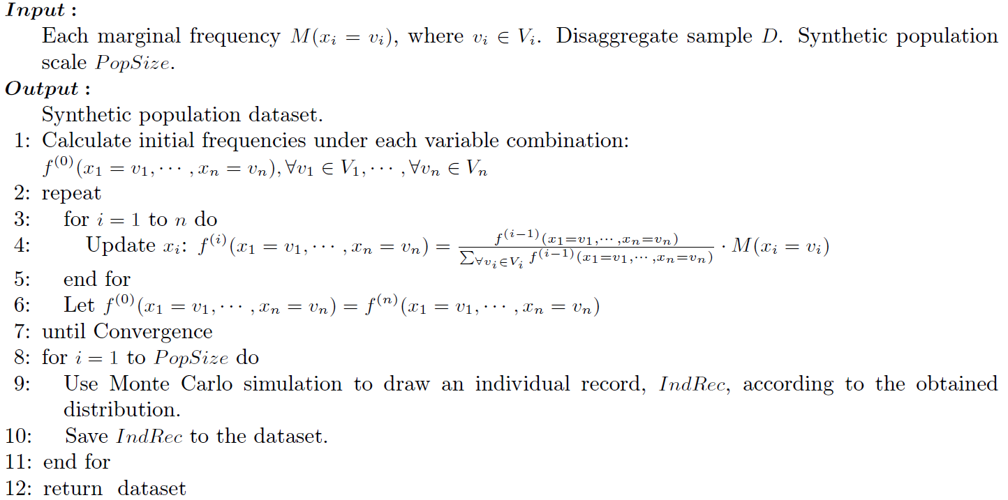
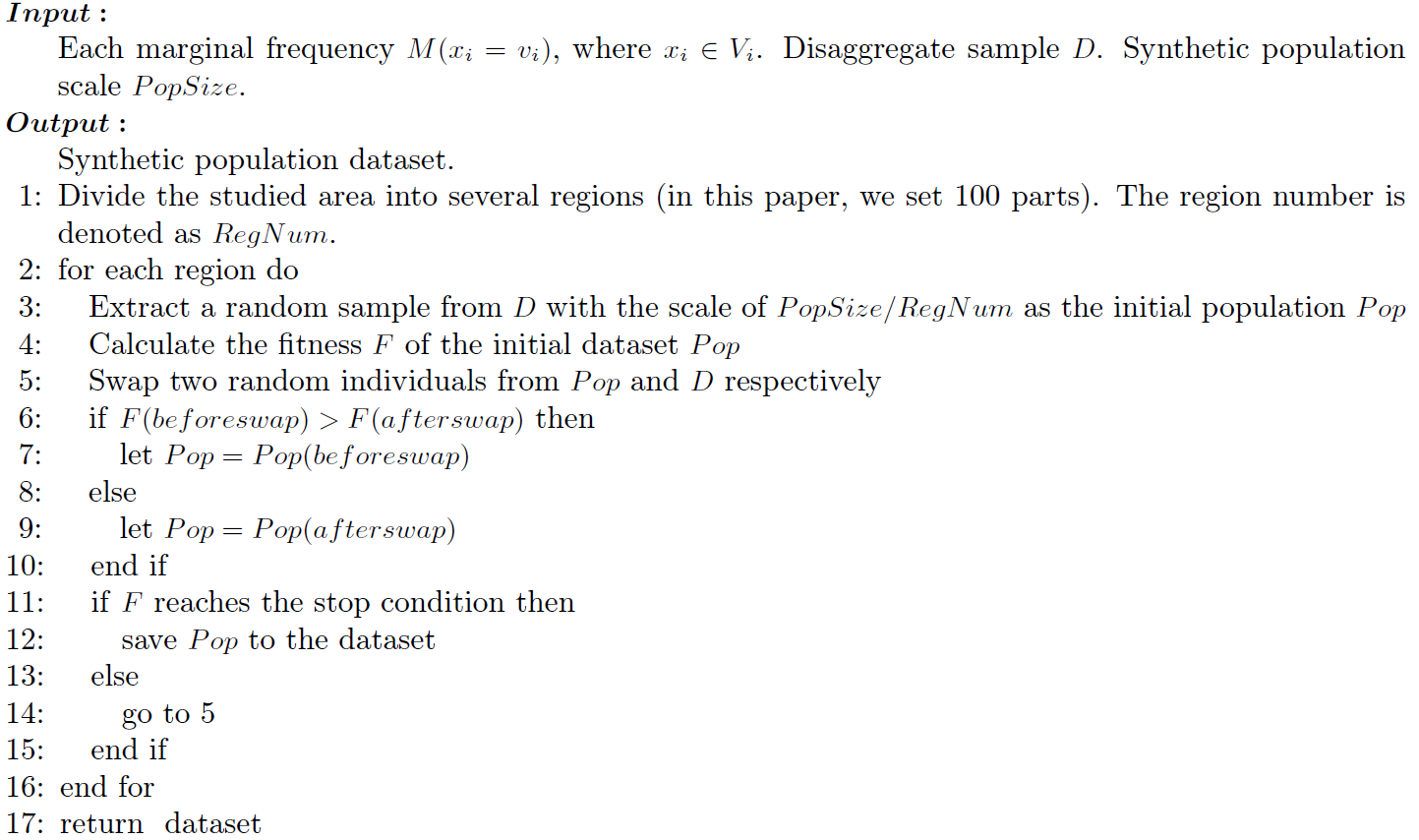
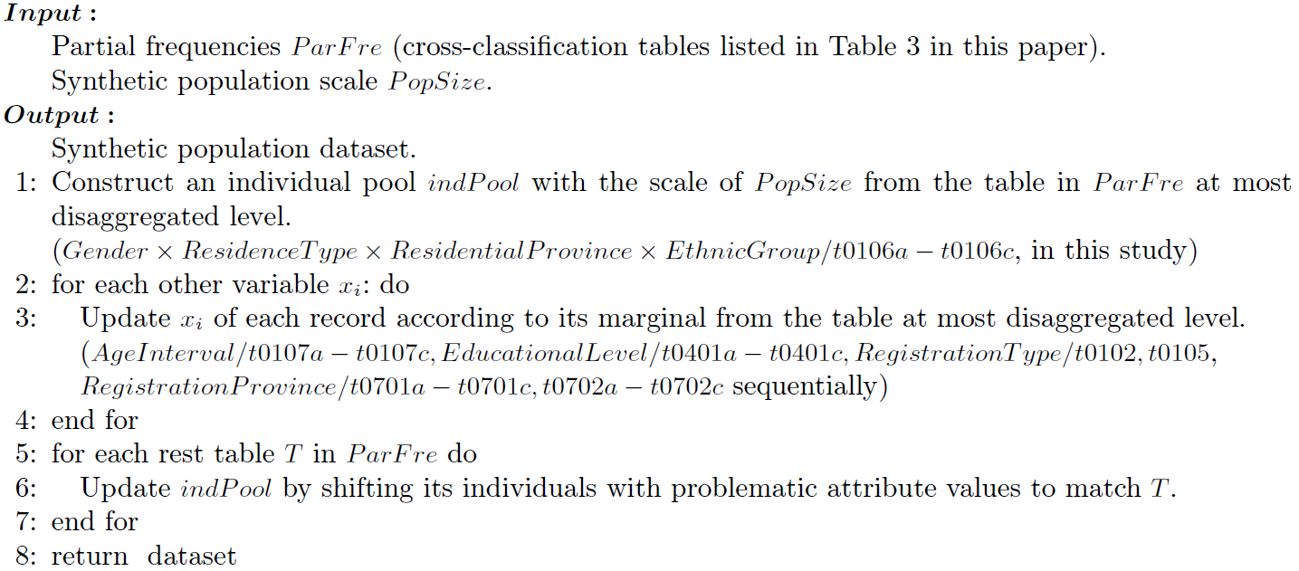
Let \(x_i(i=1,\cdots,n)\) be the variable (in this paper, \(n=8\)) with its value set \(V_i={v_j}(j=1,\cdots,d_i)\). Pseudo codes of the five algorithms are Algorithm 1 to 5.
References
ABRAHAM, J. E., Stefan, K. J. & Hunt, J. D. (2012). Population synthesis using combinatorial optimization at multiple levels. 91th Annual Meeting of Transportation Research Board, Washington DC.
ANDERSON, P., Farooq, B., Efthymiou, D. & Bierlaire, M. (2014). Associations generation in synthetic population for transportation applications graph-theoretic solution. Transportation Research Record, 2429, 38–50.
AULD, J. & Mohammadian, A. (2010). An efficient methodology for generating synthetic populations with multiple control levels. Transportation Research Record, 2175, 138–147. [doi:10.3141/2175-16]
BALLAS, D., Clarke, G., Dorling, D., Eyre, H., Thomas, B. & Rossiter, D. (2005). SimBritain: A spatial microsimulation approach to population dynamics. Population Space & Place, 11(1), 13–34.
BALLAS, D., Clarke, G., Dorling, D. & Rossiter, D. (2007). Using SimBritain to model the geographical impact of national government policies. Geographical Analysis, 39(1), 44–77. [doi:10.1111/j.1538-4632.2006.00695.x]
BARTHELEMY, J. (2014). A parallelized micro-simulation platform for population and mobility behavior-Application to Belgium. Ph.D. thesis, University of Namur.
BARTHELEMY, J. & Toint, P. L. (2013). Synthetic population generation without a sample. Transportation Science, 47(2), 266–279. [doi:10.1287/trsc.1120.0408]
BECKMAN, R. J., Baggerly, K. A. & McKay, M. D. (1996). Creating synthetic baseline populations. Transportation Research Part A, 30(6), 415–429.
CASATI, D., Muller, K., Fourie, P. J., Erath, A. & Axhausen, K. W. (2015). Synthetic population gener-ation by combining a hierarchical, simulation-based approach with reweighting by generalized raking. Transportation Research Record, 2493, 107–116. [doi:10.3141/2493-12]
DEMING, W. E. & Stephan, F. F. (1940). On a least squares adjustment of a sampled frequency table when the expected marginal totals are known. Annals of Mathematical Statistics, 11(1), 427–444.
EU (2012). A EU-funded research project: Prototypical policy impacts on multifunctional activities in rural municipalities: http://prima.cemagref.fr/.
FAROOQ, B., Bierlaire, M., Hurtubia, R. & Flotterod, G. (2013). Simulation based population synthesis. Transportation Research Part B Methodological, 58(4), 243–263.
FIENBERG, S. E. (1970). An iterative procedure for estimation in contingency tables. Annals of Mathematical Statistics, 41(3), 907–917. [doi:10.1214/aoms/1177696968]
GARGIULO, F., Ternes, S., Huet, S. & Deffuant, G. (2010). An iterative approach for generating statistically realistic populations of households. PLoS ONE, 5(1), e8828–e8828.
GEARD, N., McCaw, J. M., Dorin, A., Korb, K. B. & McVernon, J. (2013). Synthetic population dynamics: A model of household demography. Journal of Artificial Societies and Social Simulation, 16(1), 8: https://www.jasss.org/16/1/8.html. [doi:10.18564/jasss.2098]
GUO, J. Y. & Bhat, C. R. (2007). Population synthesis for microsimulating travel behavior. Transportation Research Record, 2014, 82–101.
HARDING, A., Lloyd, R., Bill, A. & King, A. (2004). Assessing poverty and inequality at a detailed regional level. Access & Download Statistics.
HARLAND, K., Heppenstall, A., Smith, D. & Birkin, M. (2012). Creating realistic synthetic populations at varying spatial scales: A comparative critique of population synthesis techniques. Journal of Artificial Societies and Social Simulation, 15(1), 1: https://www.jasss.org/15/1/1.html. [10.18564/jasss.1909]
HELLWIG, O. & Lloyd, R. (2000). Sociodemographic barriers to utilisation and participation in telecommunications services and their regional distribution: A quantitative analysis. Report, National Center for Social and Economic Modeling (NATSEM), University of Canberra.
HUANG, Z. & Williamson, P. (2001). A comparison of synthetic reconstruction and combinatorial optimisation approaches to the creation of small-area microdata. Generic, Department of Geography, University of Liverpool.
HUYNH, N., Barthelemy, J. & Perez, P. (2016). A heuristic combinatorial optimisation approach to synthesising a population for agent based modelling purposes. Journal of Artificial Societies and Social Simulation, 19(4), 11: https://www.jasss.org/19/4/11.html. [doi:10.18564/jasss.3198]
IRELAND, C. T. & Kullback, S. (1968). Contingency tables with given marginals. Biometrika, 55(1), 179–188
KING, A., McLellan, J. & Lloyd, R. (2002). Regional microsimulation for improved service delivery in Australia: Centrelink’s cusp model. In 27th General Conference, International Association for Research in Income and Wealth, (pp. 1–28).
LENORMAND, M. & Deffuant, G. (2013). Generating a synthetic population of individuals in households: Sample-free vs sample-based methods. Journal of Artificial Societies and Social Simulation, 16(4), 12: https://www.jasss.org/16/4/12.html. [10.18564/jasss.2319]
LITTLE, R. J. A. & Wu, M.-M. (1991). Models for contingency tables with known margins when target and sampled populations differ. Journal of the American Statistical Association, 86(413), 87–95. [doi:10.1080/01621459.1991.10475007]
MA, L. & Srinivasan, S. (2015). Synthetic population generation with multilevel controls: A fitness-based synthesis approach and validations. Computer-Aided Civil and Infrastructure Engineering, 30(2), 135– 150.
MELHUISH, T., Blake, M. & Day, S. (2002). An evaluation of synthetic household populations for census collection districts created using spatial microsimulation techniques. Australasian Journal of Regional Studies, 8(3),
MULLER, K. & Axhausen, K. W. (2011). Hierarchical ipf: Generating a synthetic population for Switzerland. In 51st Congress of the European Regional Science Association. Barcelona, Spain.
NBS (2000a). The 5-th national census data: http://www.stats.gov.cn/tjsj/pcsj/rkpc/5rp/index.html.
NBS (2000b). The 5-th national census questionaire: http://www.stats.gov.cn/tjsj/ndsj/renkoupucha/2000pucha/html/appen4.html>.
NBS (2010). The 6-th national census data: http://www.stats.gov.cn/english/Statisticaldata/CensusData/rkpc2010/indexch.html. [doi:10.1112/jlms/s2-21.2.379]
OU, Y., Tang, S. & Wang, F. Y. (2010). Computational experiments for studying impacts of land use on traffic systems. In Intelligent Transportation Systems (ITSC), 13th International IEEE Conference on, (pp. 1813–1818).
PRETZEL, O. (1980). Convergence of the iterative scaling procedure for non-negative matrices. Journal of the London Mathematical Society, 21(4), 379–384. [doi:10.1007/s10479-013-1468-3]
PRITCHARD, D. R. & Miller, E. J. (2012). Advances in population synthesis: Fitting many attributes per agent and fitting to household and person margins simultaneously. Transportation, 39, 685–704.
PUKELSHEIM, F. (2014). Biproportional scaling of matrices and the iterative proportional fitting procedure. Annals of Operations Research, 215(1), 269–283. [doi:10.1111/j.1538-4632.2009.00750.x]
RUSCHENDORF, L. (1995). Convergence of the iterative proportional fitting procedure. Annals of Statistics, 23(4), 1160–1174.
RYAN, J., Maoh, H. & Kanaroglou, P. (2009). Population synthesis: Comparing the major techniques using a small, complete population of firms. Geographical Analysis, 41(2).
WHEATON, W. D., Cajka, J. C., Chasteen, B. M., Wagener, D. K., Cooley, P. C., Ganapathi, L., Roberts, D. J. & Allpress, J. L. (2009). Synthesized population databases: A us geospatial database for agent-based models. Report, Research Triangle Institute.
WILLIAMS, P. (2002). Using microsimulation to create synthetic small-area estimates from Australia’s 2001 census. Working paper, National Center for Social and Economic Modeling (NATSEM), University of Canberra.
WILLIAMSON, P., Birkin, M. & Rees, P. H. (1998). The estimation of population microdata by using data from small area statistics and samples of anonymised records. Environment & Planning A, 30(30), 785–816,
WILSON, A. G. & Pownall, C. E. (1976). A new representation of the urban system for modelling and for the study of micro-level interdependence. Area, 8(4), 246–254.
YE, P., Wang, X., Chen, C., Lin, Y. & Wang, F.-Y. (2016). Hybrid agent modeling in population simulation: Current approaches and future directions. Journal of Artificial Societies and Social Simulation, 19(1), 12: https://www.jasss.org/19/1/12.html. [10.18564/jasss.2849]
ZHAO, H., Tang, S. & Lv, Y. (2009). Generating artificial populations for traffic microsimulation. IEEE Intelligent Transportation Systems Magazine, 1(3), 22–28: http://ieeexplore.ieee.org/xpl/articleDetails.jsp?arnumber=5307989.