
Introduction
The field of opinion dynamics (OD) seeks to model the mechanisms by which opinions spread through a population. Within this context, opinions may be loosely defined as Axelrod (1997) defined culture: they are any attributes that may be altered by social influence. Recent papers have extensively covered the dominant models, ideal-typical results, and challenges facing the field of OD modeling (Sîrbu et al. 2017; Flache et al. 2017). OD is inherently a multi-disciplinary field; first authors of influential papers in the field have degrees spanning cognitive science (Deffuant et al. 2000, 2002), management science (Dandekar et al. 2013), mathematics (Holley & Liggett 1975; Salzarulo 2006; Lorenz 2010), philosophy (Hegselmann & Krause 2002), psychology (Nowak et al. 1990), physics (Galam 1997; Sznajd-Weron & Sznajd 2000; Stauffer et al. 2000; Castellano et al. 2009; Martins 2009; Martins et al. 2009), political science (Axelrod 1997), social sciences (Carley 1991; Jager & Amblard 2005), sociology (Mark 1998; Friedkin 2001; Mäs et al. 2010; Mäs & Flache 2013; Mäs et al. 2013, 2014), and statistics (DeGroot 1974) to name only a few.
OD modeling lends itself to the use of what Bonabeau (2002) called the agent-based mindset, where one describes “a system from the perspective of its constituent units” (p. 7280). Using this mindset, modelers can define the rules of interaction between individual agents within the model and allow social influence to propagate throughout the system. This allows a modeler to build complex models from relatively simple rules that are based upon theories in the psychological and sociological literature. If these outputs are realistic, the modeler has proven that the proposed rules are sufficient to generate realistic emergent behavior. In other words, that behavior can be explained by the proposed mechanism. This is best stated by Epstein (1999) in his motto for generative social science: "if you didn’t grow it, you didn’t explain its emergence" (p. 43). For the purpose of this paper, agents are any objects that populate a model implementing an agent-based mindset. This is consistent with individual agent-based models (ABM) in the taxonomy proposed by Macal (2016).
While it is possible to build continuous-time OD models, discrete-time models are more common and are thus the focus of the present paper. Discrete-time OD models map the set of \(N\) agents' opinions at time \(t\) to the set of those agents' opinions at time \(t+1\). Continuous OD models are those that map \(\mathbb{R}^N \rightarrow \mathbb{R}^N\), with individual opinions drawn from a continuous range of values, typically \([0,1]\) or \([-1,1]\). These maps may take the form of a linear transformation as seen in the repeated averaging models (Harary 1959; Abelson 1964; DeGroot 1974), a deterministic non-linear transformation as seen in the the Hegselmann-Krause (HK) bounded confidence model (Hegselmann & Krause 2002), or a stochastically-varied non-linear transformation as seen in the Deffuant-Weisbuch (DW) bounded confidence model (Deffuant et al. 2000). They may take as inputs only the vector of opinions and any model parameters, as in the basic forms of those listed above, or take additional inputs from agent characteristics such as uncertainty (Deffuant et al. 2002), vectors of arguments (Mäs & Flache 2013), or locations and personality traits (Duggins 2017).
In discrete OD models, individual opinions are drawn from a discrete set of values, typically \(\{0,1\}\) or \(\{-1,1\}\). These usually implement non-linear transformations with additional inputs from agent characteristics, often including their geographic position. Examples of discrete OD models that take this form are the voter model (Holley & Liggett 1975), the social impact theory model (Nowak et al. 1990), and the Sznajd model (Sznajd-Weron & Sznajd 2000; Stauffer et al. 2000). One discrete OD model that breaks this form is the Ising field model of Galam (1997), which solves a global optimization problem without an agent-based implementation despite defining its elements using an agent-based mindset.
The agent-based mindset, for all its strengths, can yield weaknesses. One, which explains its emergence in recent decades as a viable method of modeling, is the amount of computation required. Interactions and associated computations tend to increase exponentially as the number of agents increases. Another potential weakness is the tendency to ignore system-level elements of behavior when focusing upon agent-level behavior.
One system-level behavior of an OD model that may have a significant effect upon dynamics is the agent schedule: which agent(s), in what order, influence (or are influenced by) which other agents in each discrete step of time. OD models have used various schedules with little justification. The Sznajd model has 2 agents simultaneously influencing their immediate neighbors in 1 dimension (Sznajd-Weron & Sznajd 2000; Stauffer et al. 2000). The repeated averaging models have all agents simultaneously being influenced by all others to whom they are connected (Harary 1959; Abelson 1964; DeGroot 1974). The bounded confidence models have 1 pair of agents influencing one another simultaneously in the DW model (Deffuant et al. 2000) or all agents simultaneously being influenced by all others in the HK model (Hegselmann & Krause 2002), subject to confidence constraints.
Research into the impact of varying agent schedules is limited. Cellular automata (CA) researchers have examined the effects of varying agent schedules upon CA behavior (Page 1997; Cornforth et al. 2005) and proposed schedules based on probabilistic sets of cells acting each turn and imperfect communication of states between cells at each turn (Bouré et al. 2012). A thorough survey of existing work on the impact of scheduling upon CA behavior is provided by Fatès (2014).
The world of ABM has focused much less upon this impact. The earliest ABMs, run without computers, did not adhere to any schedule strictly (Schelling 1971). In many of the most influential ABMs, all agents act in random order (examples include Holland 1995; Epstein & Axtell 1996; Epstein 2006), and books detailing the use of ABM continue to use this schedule without explanation (Gilbert & Troitzsch 2005; North & Macal 2007). Introductory tutorials on ABM tend to avoid the question of agent scheduling entirely (Bonabeau 2002; Axelrod & Tesfatsion 2006; Macal&North 2014; Macal 2016; Weimer et al. 2016). Textbooks address the difference between synchronous and asynchronous update schedules without acknowledging the variety of schedules that fit into those broad categories (Railsback & Grimm 2011; Wilensky & Rand 2015). None of these resources delve into the depth of schedules that may exist.
Research into the impact of scheduling upon ABMs is limited to a small handful of articles. Caron-Lormier et al. (2008) used a basic ecological ABM to show a significant difference in the behavior of the model when switching between two schedules. Fatès & Chevrier (2010) compared the behavior of a basic ABM based upon various deconfliction rules paired with a particular synchronous schedule and found significant differences. Bonnell et al. (2016) used a basic foraging model to examine the combined effects of cell size, cell heterogeneity, and two specific schedules upon patterns of behavior; they found significant non-linear effects and interactions between these inputs.
Notably in OD modeling, Urbig et al. (2008) generalized the DW and HK bounded confidence models into a single model where all agents are simultaneously influenced by up to \(m\) others simultaneously. They found that the general behavior of the models is qualitatively similar, although the value of \(m\) did have various effects on the specifics of that behavior. However, direction of influence was not addressed; agents were influenced by other agents' opinions without reciprocating influence, making the generalized model adaptable to replicate the HK model but not the DW model.
The Overview, Design concepts, Details (ODD) protocol (Grimm et al. 2010) encourages ABM modelers to explicitly specify the schedule used in the model. More recently, Collins et al. (2015) called for development of descriptive standards for agent-based models, but as yet no standard exists with which to communicate agent schedules in a way that is adequate for OD modeling. Some attempts at this do exist; one example focused specifically upon cellular automata is that of Cornforth et al. (2005). However, it is insufficient to adequately explain an OD model’s schedule due to not addressing direction of influence and adhering to only the extremes of scale in which one or all agents act per time step.
 |
| OD Model | Schedule Used |
| DeGroot (1974) | Synchronous Target (∞,∞) |
| Holley & Liggett (1975) | Synchronous Target (1,∞) |
| Nowak et al. (1990) | Synchronous Target (233, ∞) |
| Carley (1991) | Synchronous Group (2, ∞) |
| Axelrod (1997) | Asynchronous Target (4; 1) |
| Mark (1998) | Synchronous Group (2, ∞) |
| Friedkin (1999) | Synchronous Target (∞,∞) |
| Deffuant et al. (2000) | Asynchronous Group (2, 1) |
| Sznajd-Weron & Sznajd (2000) | Synchronous Source (2, 1) |
| Stauffer et al. (2000) | Synchronous Source (2, 3) |
| Friedkin (2001) | Synchronous Target (∞,∞) |
| Hegselmann & Krause (2002) | Synchronous Target (∞,∞) |
| Jager & Amblard (2005) | Synchronous Group (2, 1) |
| Salzarulo (2006) | Asynchronous Target (∞,1) |
| Martins et al. (2009) | Asynchronous Target (1, 1) |
| Mäs et al. (2010) | Synchronous Target (∞,1) |
| Lorenz (2010) | Synchronous Target (∞,∞) |
| Dandekar et al. (2013) | Synchronous Target (∞,∞) |
| Mäs et al. (2013) | Asynchronous Target (1, 1) |
| Mäs & Flache (2013) | Asynchronous Target (1, 1) |
| Mäs et al. (2014) | Synchronous Target (∞, 1) |
| Duggins (2017) | Asynchronous Target (∞,∞) |
The purpose of this paper is threefold: (1) to build a taxonomy for agent scheduling that is adequate for describing OD model schedules, (2) to demonstrate the potential impact of various schedules using influential continuous OD models, and (3) to discuss social interpretations of schedule choices. This taxonomy also serves to potentially unite disparate models implementing similar assumptions, such as the bounded confidence models, into a single set of parameters as recently called for by Flache et al. (2017).
Synchrony, Actor type, Scale (SAS) Scheduling Taxonomy
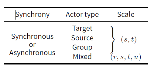
The Synchrony, Actor type, Scale (SAS) taxonomy is a concise method of communicating the schedule of an OD model. The components should be reported in order as shown in the summary in Table 1. Synchrony relates to whether states are continuously updated as agents act and has two options: synchronous and asynchronous. Actor type relates to the direction of influence and has four options: target, source, group, and mixed. Scale relates to the number of actors chosen for each role per time step and has 2 parameters (or 4 if actor type is mixed). Each component is explained in detail below. Table 2 lists the schedules of many OD models in the literature using this taxonomy.
Synchrony
Synchrony refers to whether updates to each agent’s state occur in parallel or in series. A model in which all agent updates occur in parallel would be called synchronous. A model in which some or all agent updates occur in series would be called asynchronous.
Let \(\mathcal{A}\) be a set of ordered source-target pairs \((i,j)\), where \(i\neq j\), chosen to exhibit influence in a given time step in an OD model. Let \(f_{\mathcal{A}}:\mathbb{R}^N \rightarrow \mathbb{R}^N\) be the function that maps a vector of \(N\) opinions to the vector of \(N\) opinions after the pairs in \(\mathcal{A}\) exhibit their influence synchronously. This synchronous model cannot be broken down further. A single time step of an asynchronous model, to the contrary, can be broken into a repeated application of \(f_{\{(i,j)\}}\), in some order, for each \((i,j)\) pair in \(\mathcal{A}\). Synchronous and asynchronous models are therefore identical when \(\mathcal{A}\) consists of no more than one \((i,j)\) pair, i.e., when at most one interaction occurs per time step.
Synchrony is best illustrated using a repeated averaging model. Let \(\mathbf{x}_t\in\mathbb{R}^N\) be the row vector of opinions at time \(t\). Let \(w_{ij}\) be the weight of influence from agent \(i\) to agent \(j\), where \(w_{ii}=0\). An OD model can be formulated as an \(N\times N\) matrix \(\mathbf{P}\) where
| $$\mathbf{x}_{t+1} = \mathbf{x}_t \mathbf{P}$$ |
| $$P_{ij} = \begin{cases} 0 & \text{if } i \neq j, (i,j)\notin \mathcal{A} \\ w_{ij} & \text{if } i \neq j, (i,j) \in \mathcal{A} \\ 1 - \sum\limits_{k=1}^N w_{kj} & \text{if } i=j \end{cases} $$ |
To generate an asynchronous model, let \(\mathbf{P}^{(i,j)}\) be the \(N\times N\) matrix defining a synchronous model where \(\mathcal{A}=\{(i,j)\}\). Let \(\mathcal{A}^{(l)}\) be the \(l\)th pair drawn in some order from \(\mathcal{A}\). Then the asynchronous model is defined by
| $$ \mathbf{P} = \mathbf{P}^{\mathcal{A}^{(1)}} \mathbf{P}^{\mathcal{A}^{(2)}} \cdots \mathbf{P}^{\mathcal{A}^{(|\mathcal{A}|)}} $$ |
A synchronous model's update in an object-oriented programming language may be written as two steps: (1) update temporary opinions for each agent using the permanent opinions of other agents and (2) update permanent opinions to match temporary opinions. This avoids cascading effects within a single time step such that agent \(i\)'s opinion at time \(a\) has no effect on agent \(j\)'s opinion at time \(a+1\) unless agent \(i\) directly influences agent \(j\).
An asynchronous model updates permanent opinions directly after each interaction. This allows cascading effects within a single time step such that agent \(i\)'s opinion may influence agent \(j\)'s opinion without directly influencing agent \(j\). This occurs when there is an unbroken chain of influence between agent \(i\) and agent \(j\) in the order of agents' actions.
Actor type
In the context of the SAS taxonomy, the primary actor in an OD model is the entity that is chosen to act. In an agent-based model, this is the agent or group of agents that executes code directly. Primary actors may be paired with other agents in the course of this action. An agent paired in such a way is a secondary actor. In a model not explicitly coded as an agent-based model, the primary actor is implicitly identified as performing some action by the mathematical formulation.
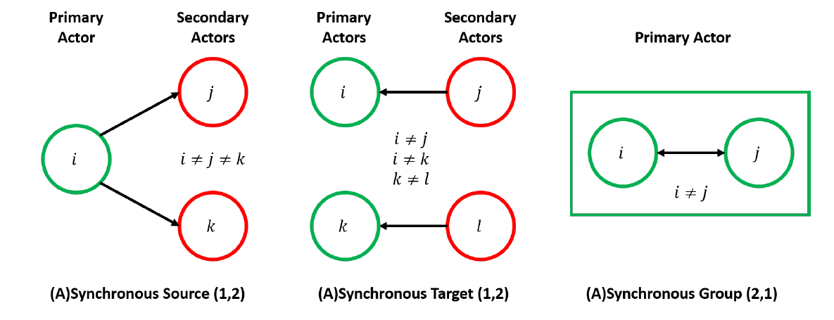
In defining a model built from an agent-based mindset, three primary actor types exist: source agents who influence others when they act, target agents who are influenced by others when they act, and groups of agents who mutually influence one another. The choice of agent type impacts the schedule both in how pairing of agents is performed and, for asynchronous schedules, the order in which influence occurs. Figure 1 shows examples of possible pairings based on actor types. Additionally, it is possible for actors to be of mixed type; various “breeds” of agent may act differently, for example, or an agent’s action may vary as a function of the model state.
If primary actors are source agents, some set of secondary actors (i.e., targets) is chosen for each primary actor. In an asynchronous model, this source influences all of its targets before another source acts. If primary actors are target agents, some set of secondary actors (i.e., sources) is chosen for each primary actor. In an asynchronous model, this target is influenced by all of its sources before another target acts.
If primary actors are groups of agents, there are no secondary actors; each group exhibits influence between member agents as defined by the model. Each group action may be represented as an OD model executed upon a subset of agents, so these schedules may be further refined using the SAS taxonomy. Deconfliction rules may be required for synchronous models when one agent may be chosen to act as a member of multiple groups.
If primary actors are of mixed types, some or all of the above actor types exist and act within the model. It must be specified whether actors of a given type act before actors of another type, representing sequential applications of multiple OD models within a time step, or they act in mixed order, representing a truly mixed OD model.
Regardless of primary actor type, it is vital for the modeler to further detail the order in which agents take action. Random order is common, but potential alternative ordering techniques are without limit.
Scale
In the context of the SAS taxonomy, scale refers to the number of agents contained in sets of primary actors, secondary actors, and groups. For a model using source actors, no more than \(s\) source agents are chosen as primary actors, with no more than \(t\) target agents selected as secondary actors for each primary actor. For a model using target actors, no more than \(t\) target agents are chosen as primary actors, with no more than \(s\) source agents selected as secondary actors for each. For a model using group actors, no more than \(t\) groups of no more than \(s\) agents each are chosen to influence one another. For a model with mixed-type actors, no more than \(r\) agents are chosen to act as primary actors. If a primary actor acts as a target, it is influenced by no more than \(s\) secondary actors; if it acts as a source, it influences no more than \(t\) secondary actors; and if it is a group, it consists of no more than \(u\) agents. Parameters should be listed in alphabetical order.
If the model imposes scaling limits below the number of agents in the model, related parameters should be given as positive integers. Otherwise, parameters should be reported as \(\infty\) to communicate the scale is not limited. This allows direct comparison between otherwise-identical models of differing population sizes. Similarly, if individual agents are heterogeneous with respect to scale parameters, the largest scale parameter should be reported along with more detail regarding those heterogeneous values.
Generalized Repeated Averaging Model
To demonstrate the use of the SAS taxonomy, and to demonstrate potential differences that may arise in model outputs as a result of differing schedules, we examine two models generalized from those available in the literature. The first of these is the repeated averaging model.
Model definition
As originally presented by (Harary 1959), the repeated averaging model uses a linear transformation upon the vector of agents' opinions to perform discrete-time updates. This linear transformation takes the form of an \(N\times N\) right-stochastic matrix of pair-wise weights between agents. DeGroot (1974) and Berger (1981) proved that this model tends to converge under reasonable conditions. We limit our model such that these conditions are met.
The generalized repeated averaging model (GRAM) removes the requirement that the model's matrix be pre-determined and static. For ease of communication, we use the transposed form of earlier models. Let \(\mathbf{x}_t\) be the row vector of agent opinions at time \(t\) and \(\mathbf{P}\) be the left-stochastic matrix defining the OD model from time \(t\) to time \(t+1\). Then,
| $$\mathbf{x}_{t+1} = \mathbf{x}_t \mathbf{P}$$ |
This matrix is further restricted to have diagonal elements of value \((1-\mu)\), where \(\mu\in (0,1)\) is a convergence parameter analogous to that in the Deffuant-Weisbuch model (Deffuant et al. 2000). An individual agent, if influenced during time \(t\), grants \(\mu\) influence to others while maintaining \((1-\mu)\) self-influence. This ensures that the model converges and allows direct comparison between varied schedules.
\(\mathbf{P}\) may vary over time as different primary and secondary actors are chosen and, in the case of asynchronous schedules, as the order of actors changes. Actors are always selected at random from the pool of available agents. As all agents are equally likely to be chosen at each time step, the social network is a complete graph. However, depending on schedule parameters, every pair of agents need not interact at each time step.
Further definition of the GRAM varies by synchrony and actor type. For precision in defining the model, it is defined in matrix form.
Synchronous
Let us first consider the model associated with a Synchronous Target \((s,t)\) schedule. Let \(\mathcal{T}\) be the set of \(t\) target agents randomly chosen as primary actors, or the set of all agents if \(t\geq N\). For each agent \(j\in\mathcal{T}\), let \(\mathcal{S}_j\) be the set of \(s\) source agents randomly chosen to influence agent \(j\), or the set of all other agents if \(s\geq N-1\). The matrix associated with the model appears as an \(N\times N\) identity matrix where columns with indices in \(\mathcal{T}\) are modified. It may be defined element-wise by
| $$\begin{align} P_{ij} &= \begin{cases} 0 & \text{if } i \neq j, j \notin \mathcal{T} \\ 1 & \text{if } i = j, j \notin \mathcal{T} \\ %0 & \text{if } j \in \mathcal{T}, i \neq j, i \notin \mathcal{S}_j \\ \frac{\mu}{|\mathcal{S}_j|} & \text{if } i \neq j, j \in \mathcal{T}, i \in \mathcal{S}_j \\ 1 - \mu & \text{if } i = j, j \in \mathcal{T},\\ 0 & \text{otherwise} \end{cases}\end{align}$$ | (1) |
For the Synchronous Source \((s,t)\) schedule, let \(\mathcal{S}\) be the set of \(s\) source agents randomly chosen as primary actors, or the set of all agents if \(s\geq N\). For each agent \(i \in \mathcal{S}\), let \(\mathcal{T}_i\) be the set of \(t\) target agents randomly chosen to be influenced by agent \(i\), or the set of all agents if \(t\geq N-1\). By extension, let \(\mathcal{S}_j\) be the set of agents \(i\) for which \(j\in \mathcal{T}_i\). The matrix associated with this model appears as an identity matrix where rows with indices in \(\mathcal{S}\) are modified. It is defined by
| $$\begin{align} P_{ij} &= \begin{cases} 0 & \text{if } i \notin \mathcal{S}, j \neq i \\ 1 & \text{if } i \notin \mathcal{S}, j = i \\ %0 & \text{if } i \in \mathcal{S}, i \neq j, j \notin \mathcal{T}_i \\ \frac{\mu}{|\mathcal{S}_j|} & \text{if } i \in \mathcal{S}, j \neq i, j \in \mathcal{T}_i \\ 1 - \mu & \text{if } i \in \mathcal{S}, j = i \\ 0 & \text{otherwise} \end{cases} \end{align}$$ | (2) |
For the Synchronous Group \((s,t)\) schedule, we assume that repeat influences may not occur; that is, if two agents are members of multiple groups, they only influence each other once. Let \(\mathcal{A}\) be the set of \(t\) \(s\)-tuples of agents chosen as primary actors, or the set of all possible \(s\)-tuples of agents if \(t\geq \binom{N}{s}\). Let \(\mathcal{T}\) be the set of all agents belonging to one or more groups in \(\mathcal{A}\). For each agent \(j\), let \(\mathcal{S}_j\) be the set of all agents belonging to one or more groups in \(\mathcal{A}\) that also contain agent \(j\). The matrix associated with this model is defined by
| $$\begin{align} P_{ij} &= \begin{cases} 0 & \text{if } i \neq j, j \notin \mathcal{T} \\ 1 & \text{if } i = j, j \notin \mathcal{T} \\ %0 & \text{if } j \in \mathcal{T}, i \neq j, i \notin \mathcal{S}_j \\ \frac{\mu}{|\mathcal{S}_j|} & \text{if } i \neq j, i \in \mathcal{S}_j, j \in \mathcal{T} \\ 1 - \mu & \text{if } i = j, j \in \mathcal{T} \\ 0 & \text{otherwise} \end{cases} \end{align}$$ | (3) |
Mixed actor types are not used in the GRAM. The multitude of options make direct comparison to other actor types impossible. Furthermore, we are not aware of any OD models that have used mixed actor types.
Asynchronous
Asynchronous schedules are more complicated to define as a result of their iterative nature. Let us first define the matrix \(\mathbf{P}^{(i,j)}\), which is used for both source and target actor types. This is the matrix associated with a Synchronous Target (1,1) GRAM where \(\mathcal{T}=\{j\}, \mathcal{S}_j = \{i\}, \mu=\mu^*\).
To solve for the appropriate value of \(\mu^*\), we must ensure that \((1-\mu)\) influence remains assigned to the agent's initial opinion at the end of the time step, potentially after several iterative updates. Consider agent \(j\), with a set of source agents \(\mathcal{S}_j\) that will serially influence agent \(j\) in some order. Let \(\mathcal{S}_j^{(k)}\) be the \(k\)th element drawn from \(\mathcal{S}_j\). The opinion of agent \(j\) (\(x_j\)) after the \(k\)th interaction becomes
| $$\begin{align} x_j &\leftarrow (1-\mu^*) \cdot x_j + \mu^* \cdot x_{\mathcal{S}_j^{(k)}} \end{align} $$ | (4) |
| $$\begin{align} x_j &\leftarrow (1-\mu^*)^{|\mathcal{S}_j|}\cdot x_j + \sum\limits_{k=1}^{|\mathcal{S}_j|}\left((1-\mu^*)^{|\mathcal{S}_j|-k}\cdot\mu^* \cdot x_{\mathcal{S}_j^{(k)}} \right) \end{align}$$ | (5) |
In order to maintain \((1-\mu)\) self-influence, we then have that
| $$\begin{align} (1-\mu^*)^{|\mathcal{S}_j|} = (1-\mu) &\implies \mu^* = 1 - (1-\mu)^{\frac{1}{|\mathcal{S}_j|}} \end{align}$$ | (6) |
The matrix \(\mathbf{P}^{(i,j)}\) is therefore defined as
| $$\begin{align} P^{(i,j)}_{kl} &= \begin{cases} 0 & \text{if } k \neq l, l \neq j \\ 1 & \text{if } k = l, l \neq j \\ 1 - (1-\mu)^{\frac{1}{|\mathcal{S}_j|}} & \text{if } k \neq l, l = j \\ (1-\mu)^{\frac{1}{|\mathcal{S}_j|}} & \text{if } k = l = j \\ 0 & \text{otherwise} \end{cases} \end{align}$$ | (7) |
We may now define the Asynchronous Target \((s,t)\) GRAM. Let \(\mathcal{T}\) be the set of \(t\) target agents randomly chosen as primary actors, or the set of all agents if \(t\geq N\). For each agent \(j\in\mathcal{T}\), let \(\mathcal{S}_j\) be the set of \(s\) source agents randomly chosen to influence agent \(j\), or the set of all other agents if \(s\geq N-1\). Let \(\mathcal{T}^{(l)}\) be the \(l\)th element drawn from \(\mathcal{T}\), and let \(\mathcal{S}_j^{(k)}\) be the \(k\)th element drawn from \(\mathcal{S}_j\). The matrix associated with the model, then, is the ordered product of \(\mathbf{P}^{(i,j)}\) matrices.
| $$\begin{align} \mathbf{P} &= \prod\limits_{l=1}^{|\mathcal{T}|} \prod\limits_{k=1}^{|\mathcal{S}_l|} \mathbf{P}^{\left(\mathcal{S}_{\mathcal{T}^{(l)}}^{(k)},\mathcal{T}^{(l)}\right)} \label{eq:AsyncTargP} \end{align} $$ | (8) |
For the Asynchronous Source \((s,t)\) GRAM, let \(\mathcal{S}\) be the set of \(s\) source agents randomly chosen as primary actors, or the set of all agents if \(s\geq N\). For each agent \(i\in\mathcal{S}\), let \(\mathcal{T}_i\) be the set of \(t\) target agents randomly chosen to be influenced by agent \(i\), or the set of all other agents if \(t\geq N-1\). By extension, let \(\mathcal{S}_j\) be the set of agents \(i\) for which \(j\in \mathcal{T}_i\). Let \(\mathcal{S}^{(k)}\) be the \(k\)th element drawn from \(\mathcal{S}\), and let \(\mathcal{T}_i^{(l)}\) be the \(l\)th element drawn from \(\mathcal{T}_i\). The matrix associated with the model is again the ordered product of \(\mathbf{P}^{(i,j)}\) matrices.
| $$\begin{align} \mathbf{P} &= \prod\limits_{k=1}^{|\mathcal{S}|} \prod\limits_{l=1}^{|\mathcal{T}_k|} \mathbf{P}^{\left(\mathcal{S}^{(k)},\mathcal{T}_{\mathcal{S}^{(k)}}^{(l)}\right)} \label{eq:AsyncSourP} \end{align} $$ | (9) |
For the Asynchronous Group \((s,t)\) GRAM, let \(\mathcal{A}\) be the set of \(t\) \(s\)-tuples of agents chosen as primary actors, or the set of all possible \(s\)-tuples of agents if \(t\geq \binom{N}{s}\). Let \(\mathcal{A}^{(k)}\) be the \(k\)th element drawn from \(\mathcal{A}\). Let \(\mathbf{P}^{\mathcal{A}^{(k)}}\) be the matrix associated with a Synchronous Group \((s,1)\) GRAM where \(\mathcal{A}^{(k)}\) is the chosen primary actor according to Equation 3. The Asynchronous Group \((s,t)\) GRAM's associated matrix is the ordered product of \(\mathbf{P}^{\mathcal{A}^{(k)}}\) matrices.
| $$\begin{align} \mathbf{P} &= \prod\limits_{k=1}^{|\mathcal{A}|} \mathbf{P}^{\mathcal{A}^{(k)}} \label{eq:AsyncGrpP} \end{align} $$ | (10) |
Parameter selection
Parameters for the GRAM that remain in need of values are \(s\), \(t\), \(\mu\), and \(N\). The intent of the present experiment is to motivate experimenters to explicitly state their schedule use by showing that scheduling choices can have a significant impact upon the outcome of an OD model. Therefore, a quantity of interest is the influence that particular agents have based on their order in an asynchronous model.
In an Asynchronous Target \((s,t)\) schedule, let the coefficient associated with agent \(i\)'s influence upon agent \(j\) be denoted \(\lambda_i\). As shown in Equation 5,
| $$\begin{align} \lambda_i &= (1-\mu^*)^{|\mathcal{S}_j|-k} \cdot \mu^* = (1-\mu)^{\frac{|\mathcal{S}_j|-k}{|\mathcal{S}_j|}} \cdot \left( 1 - (1-\mu)^{\frac{1}{|\mathcal{S}_j|}} \right) \label{eq:Lambda} \end{align} $$ | (11) |
| $$\begin{align} \lambda_{|\mathcal{S}_j|} - \lambda_1 &= 2 - \mu - (1-\mu)^\frac{1}{|\mathcal{S}_j|} - (1-\mu)^{1 - \frac{1}{|\mathcal{S}_j|}} \label{eq:LambdaDiff} \end{align}$$ | (12) |
For a set value of \(\mu\), this is a decreasing function of \(|\mathcal{S}_j|\) when \(|\mathcal{S}_j|\geq 2\) and equals \(0\) when \(|\mathcal{S}_j| = 1\). Therefore, the greatest absolute difference in influence is observed when \(s=|\mathcal{S}_j|=2\).
| $$\begin{align} \max_{|\mathcal{S}_j|}{\lambda_{|\mathcal{S}_j|} - \lambda_1} &= \left(1 - \sqrt{1-\mu}\right)^2 \end{align}$$ | (13) |
Using the same schedule, another measure of interest would be the ratio of the last agent’s influence to that of the first. From Equation 11 we can calculate this ratio.
| $$\begin{align} \frac{\lambda_{|\mathcal{S}_j|}}{\lambda_1} &= (1-\mu)^{\frac{1}{|\mathcal{S}_j|} - 1} \label{eq:LambdaRatio} \end{align}$$ | (13) |
Because \(\mu\in(0,1)\), for a set value \(\mu\), this is an increasing function of \(|\mathcal{S}_j|\) with value \(1\) when \(|\mathcal{S}_j|=1\) that approaches \((1-\mu)^{-1}\) as \(|\mathcal{S}_j|\rightarrow\infty\). For a set value of \(|\mathcal{S}_j|\), this is an increasing function that approaches \(0\) as \(\mu\rightarrow0^+\) and approaches \(\infty\) as \(\mu\rightarrow1^-\). Therefore, the greatest influence ratio is observed when \(s=\infty\) and \(\mu\) is large.
In an Asynchronous Source \((s,t)\) schedule, the precise influence of an agent is not analytically tractable because effects cascade depending upon the nature of the social network defined by primary and secondary actor selection. Some observations related to order may still be made, however. The first primary actor shifts the mean opinion in the model toward their opinion upon action. If one of that actor's secondary actors is a later primary actor, that shift further affects the mean. The probability of this occurring increases with \(t\). Therefore, we expect the influence of an agent \(i\) to decrease with \(k\), the order in which agent \(j\) is drawn from \(\mathcal{S}\). Furthermore, we expect this variation in influence to increase with \(t\). Because the opinion of source agent \(i\) is unchanging, the order in which agents are drawn from \(\mathcal{T}_i\) has no effect.
In an Asynchronous Group \((s,t)\) schedule, as defined in the GRAM, cascading effects behave similarly to those in the Asynchronous Source \((s,t)\) schedule. Therefore, we expect the influence of agents in group \(k\), where \(k\) is the order in which that group of agents is drawn from \(\mathcal{A}\), to decrease as \(k\) increases. The probability of cascading effects increases with \(t\), again, so we also expect the difference in influence to increase with \(t\). Note that when \(s=\infty\), only one group is possible (all agents), so the Asynchronous Group \((\infty,t)\) GRAM is identical to the Synchronous Target \((\infty,\infty)\), the Synchronous Source \((\infty,\infty)\), and the Synchronous Group \((\infty,\infty)\) GRAMs.
These results suggest that \(s\) should be varied between \(2\) and \(\infty\) for Source and Target actor types and held at \(2\) for Group actors. Because there is no reason to believe that \(t\) would have a significant effect for Source actors while high values of \(t\) elicit the most effect for Target and Group actors, \(t\) should be set high for those actor types. Increasing \(t\) beyond \(1000\) has no effect upon models with Source and Target actors, but increasing \(t\) has an effect up to \(\binom{N}{s}\) for Group actors, so setting \(t=1000\) allows for the most direct comparisons between actor types by keeping the number of total interactions equal. Furthermore, although we expect the greatest magnitude of effect when \(\mu\) is high, a range of values should be examined to assess the robustness of these findings. The number of agents, \(N\), should be set to a high value, but computation time increases exponentially with \(N\). Informal pilot runs varying \(N\) indicated \(N=1000\) is a good compromise value. Thus, all simulations are performed with \(t=1000,N=1000\), \(s\) varied between \(2\) and \(1000\), and \(\mu\) varied from \(0.01\) to \(0.99\) at increments of \(0.01\) \(t=1000,N=1000\), \(s\) varied between \(2\) and \(1000\), and \(\mu\) varied from \(0.01\) to \(0.99\) at increments of \(0.01\).
The order effects also suggest a manner of observing the impact that schedule may have by biasing that order. Randomly ordering agent actions should obscure any variance in influence when a large number of agents are used. However, there is no reason to believe that humans are influenced in random order by those with whom they interact. Indeed, the dynamics of individual conversations is a relatively unexplored area in opinion dynamics (Duggins 2017 is a notable exception here). To showcase the most extreme potential effect that scheduling may have, randomized order (i.e., unbiased) and biased order models are compared for asynchronous schedules. Bias toward 0 may be induced by ordering agent actions in a particular way. When primary actors are targets, sources acting in order of decreasing opinion induces negative bias; Equations 12 and 14 show that later sources have higher influence. When primary actors are sources, acting in order of increasing opinions induces negative bias; early actors’ influence has an opportunity to cascade more than later actors’ influence. Similarly, when primary actors are groups, acting in increasing order of the mean opinions of agents within the group induces negative bias.
Results
The GRAM was run for 1000 replications for each set of parameters, beginning with a set of N = 1000 agents initialized to uniformly distributed opinions. It is considered to have converged when the range of opinions falls below 0.01.
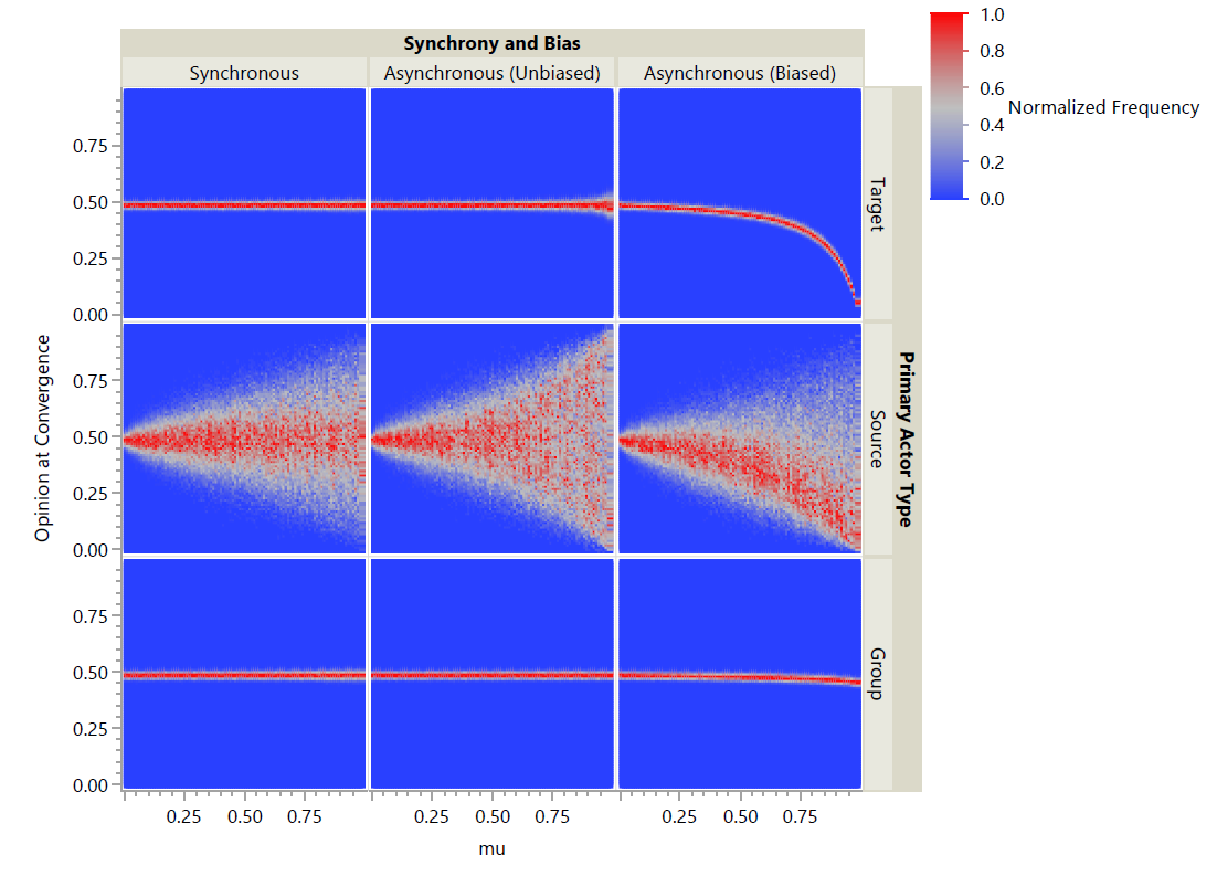
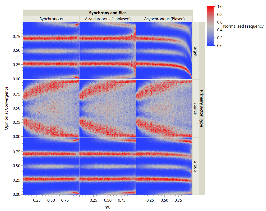
Normalized heat maps are shown in Figure 2 and Figure 3. For each set of parameters (seen as a column within a plot), the associated histogram was generated for bins of width 0.01 and frequencies were normalized such that a value of 0 is observed only if no outcome resulted in that opinion and a value of 1 is observed only if that opinion was the most frequently observed outcome for that set of parameters. Each dot in these plots is colored according to the normalized frequency, with red being the most common outcome and blue being unseen outcomes.
For s = 2, all three primary actor types (target, source, group) were examined with and without synchrony. When schedules were asynchronous, both unbiased and biased forms were run as described above. Figure 2 shows the results as a normalized heat map. This broad view shows that there are differences between schedules with respect to the degree of biasing exhibited in biased models and the variance in observed opinions at convergence. Both source and target primary actors exhibited noticeable differences in variance for high values of \(\mu\) when changing synchrony. For all synchrony and biases, source primary actors generate drastically higher variance in opinions at convergence than target or group primary actors. Group primary actors exhibit the weakest biasing with relatively small variance even for high μ.
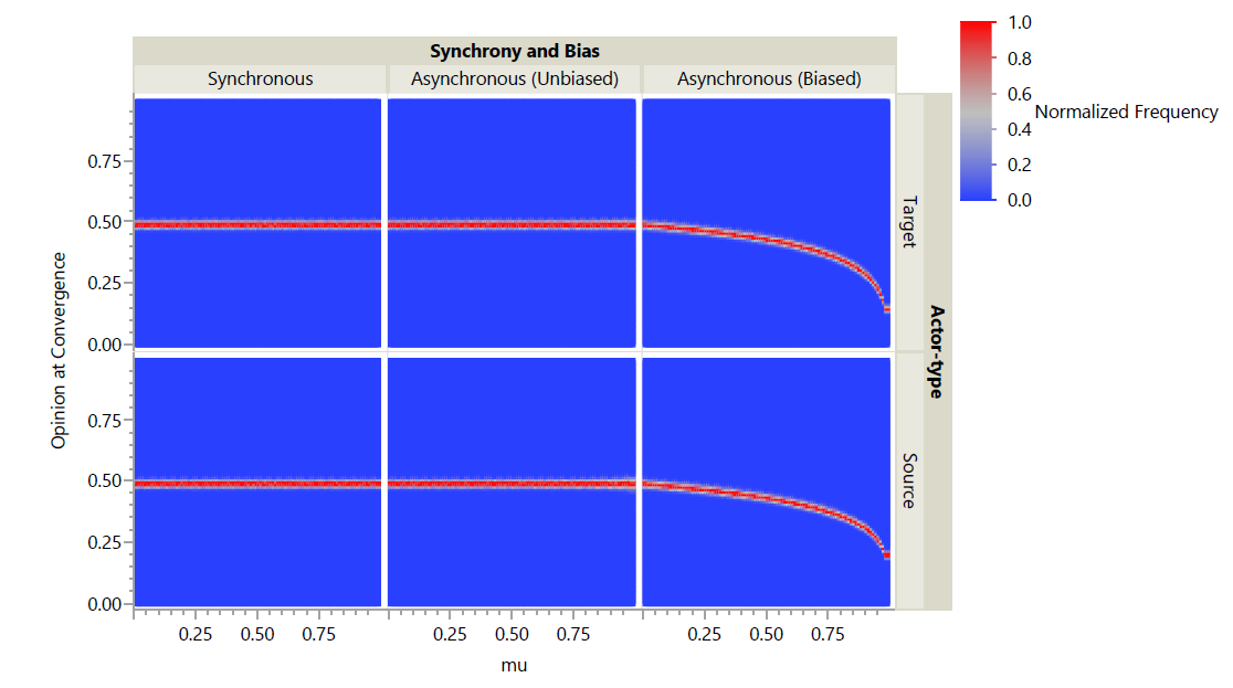
For \(s=\infty), only source and target primary actors were simulated; as the action for group primary actors is defined, those models would be equivalent for both synchronous and asynchronous schedules. Furthermore, for synchronous schedules, source and target primary actors result in identical models; therefore, only target primary actors were simulated, although the results show them in both positions for ease of comparison. When schedules were asynchronous, both unbiased and biased forms were again run. Figure 3 shows the results as a normalized heat map. A larger value of s appears from a broad view to have eliminated the differences between schedules. A closer view is warranted.
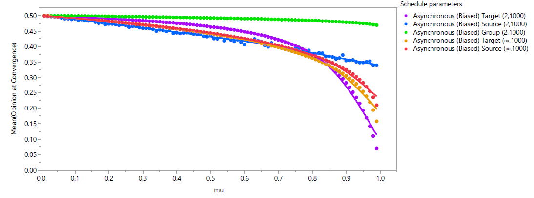
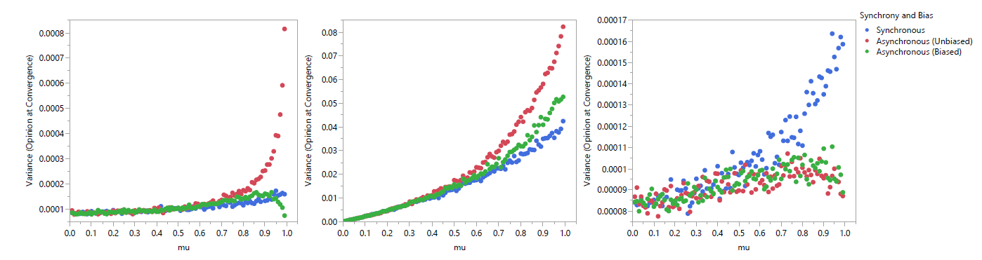
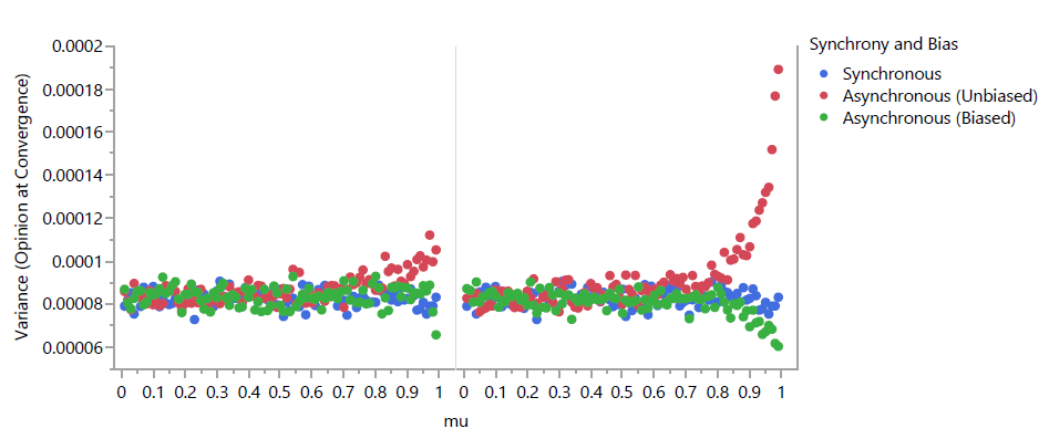
Figure 4 (for \(s = 2\)) and 5 (for \(s=\infty\)) plot the variance observed for each parameter set across 1000 replicates. Note that scales vary between plots in Figure 4 due to the drastic differences in scale between actor types that mostly disappear for \(s=\infty\). The variance in observed opinions for the Source \((2,1000)\) schedules stands out as being significantly different from that observed with other schedules. This is likely due to the strong influence that the first agents chosen have upon every other agent. However, closer examination shows that all schedules exhibit unique patterns of variance as \(\mu\) is varied. Interestingly, increasing \(\mu\) beyond a point for some schedules actually has the effect of decreasing variance. For the biased Asynchronous Target \((2,1000)\), biased Asynchronous Target \((\infty,1000)\), and biased Asynchronous Source \((\infty,1000)\) models, this is likely the result of the strength of schedule bias overcoming other sources of variance. For the Asynchronous Group \((2,1000)\) schedules, we suspect that the cohesive impact of high values of \(\mu\) decreases the variance based upon early interactions of agents with disparate opinions that moderate both agents.
The biasing effect of ordering primary actors according to their opinion can be clearly observed in the results in Figure 6, a plot of the mean observed outcomes across all \(1000\) replicates for each parameter setting for which bias is included. As expected, bias is strongest when the convergence parameter \(\mu\) is high, but it is clearly observable even for low to moderate values. When \(\mu<0.65\), the schedule that exhibits the strongest bias is the Asynchronous Source \((2,1000)\). In this schedule, the mean opinion at convergence decreases in a nearly linear fashion as \(\mu\) increases, while other schedules exhibit more nonlinear effects. When \(0.65\leq\mu\leq 0.85\), the strongest bias is exhibited in the Asynchronous Target \((\infty,1000)\) schedule. For \(\mu>0.85\), the strongest bias is in the Asynchronous Target \((2,1000)\) schedule. For all values of \(\mu\), biasing is weakest with an Asynchronous Group \((2,1000)\) schedule.
Generalized Bounded Confidence Model
While the GRAM is sufficient to demonstrate differences that may arise in model outputs as a result of schedule selection, there is value in presenting results for a more complex model in more common contemporary usage. The bounded confidence OD models presented by Deffuant et al. (2000) (the Deffuant-Weisbuch or DW model) and that presented by Hegselmann & Krause (2002) (the Hegselmann-Krause or HK model) have been heavily studied and reused. The two are very similar to one another; the primary difference relates to schedule. Using the SAS taxonomy, the DW model uses a Asynchronous Group \((2,1)\) schedule while the HK model uses a Synchronous Target \((\infty,\infty)\) schedule.
The generalized bounded confidence model (GBCM) is a generalized model that includes the DW, but not the HK model, as a special case. Taking an average of all agents within confidence threshold \(d\), as the HK model does, sets individual values of \(\mu\) to \(\frac{\mathcal{S}_j-1}{\mathcal{S}_j}\). Thus, including the HK model perfectly into the GBCM would negate the ability to compare between schedules as \(\mu\) would become heterogeneous between agents, and its scale would vary with actor type and scale parameters. A near analogue exists, however, using the same schedule but fixing \(\mu\) as a homogeneous input parameter.
The GBCM differs from the GRAM in one key way: after initializing sets \(\mathcal{S}_j\) and/or \(\mathcal{T}_i\), they are filtered to only include secondary actors whose opinions are within \(d\) of the primary actor, where \(d\) is the confidence threshold. In order to include the base DW and HK models and enable direct comparisons between schedules, \(d\) is homogeneous across the model.
Model definition
The above informal definition of the model is useful for a conceptual overview of the GBCM but insufficiently precise to replicate the model. Let \(\mathbf{x}_t\) again be the row vector of \(N\) agent opinions at time \(t\) and \(\mathbf{P}\) be the left-stochastic \(N \times N\) matrix defining the OD model from time \(t\) to \(t+1\). Then,
| $$\mathbf{x}_{t+1} = \mathbf{x}_t\mathbf{P}$$ |
As with the GRAM, \(\mathbf{P}\) is further restricted to have diagonal elements of value \((1-\mu)\), where \(\mu\in(0,1)\) is a convergence parameter. An individual agent, if influenced during time \(t\), grants \(\mu\) influence to others while maintaining \((1-\mu)\) self-influence. This form ensures the clusters converge and allows direct comparison between schedules.
Again, \(\mathbf{P}\) may vary over time as sets of primary and secondary actors are chosen and, in the case of asynchronous schedules, as the order of actors changes. Actors are always initially selected at random from the pool of available agents, regardless of their opinions.
Further definition of the GBCM varies by synchrony and actor type. For precision in defining the model, it is defined in matrix form.
Synchronous
For the Synchronous Target \((s,t)\) schedule, let \(\mathcal{T}\) be the set of \(t\) target agents randomly chosen as primary actors, or the set of all agents if \(t\geq N\). For each agent \(j\in \mathcal{T}\), let \(\mathcal{S}_j^*\) be the set of \(s\) source agents randomly chosen to potentially influence agent \(j\), or the set of all other agents if \(s\geq N-1\). Let \(\mathcal{I}_j\) be the set of agents \(i\) for whom \(|x_i - x_j| \leq d\). The set \(\mathcal{S}_j = \mathcal{S}_j^* \cap \mathcal{I}_j\) becomes the filtered set of eligible sources. The matrix \(\mathbf{P}\) associated with the model is the \(N \times N\) matrix derived from \(\mathcal{T}\) and \(\mathcal{S}_j\) that is defined by Equation 1.
For the Synchronous Source \((s,t)\) schedule, let \(\mathcal{S}\) be the set of \(s\) source agents randomly chosen as primary actors at time \(t\), or the set of all agents if \(s\geq N\). For each agent \(i\in \mathcal{S}\), let \(\mathcal{T}_i^*\) be the set of \(t\) target agents randomly chosen to potentially be influenced by agent \(i\), or the set of all other agents if \(t\geq N-1\). Let \(\mathcal{I}_i\) be the set of agents \(j\) for whom \(|x_i - x_j| \leq d\). The set \(\mathcal{T}_i = \mathcal{T}_i^* \cap \mathcal{I}_i\) becomes the filtered set of eligible targets. By extension, let \(\mathcal{S}_j\) be the set of agents \(i\) for which \(j\in \mathcal{T}_i\). The matrix \(\mathbf{P}\) associated with the model is the \(N \times N\) matrix derived from \(\mathcal{S}\) and \(\mathcal{S}_j\) that is defined by Equation 2.
For the Synchronous Group \((s,t)\) schedule, we again assume that repeat influences may not occur. Let \(\mathcal{A}\) be the set of \(t\) \(s\)-tuples of agents initially chosen as primary actors, or the set of all possible \(s\)-tuples of agents if \(t\geq \binom{N}{s}\). Let \(\mathcal{T}\) be the set of all agents belonging to one or more groups in \(\mathcal{A}\). For each agent \(j\), let \(\mathcal{S}_j^*\) be the set of all agents belonging to one or more groups in \(\mathcal{A}\) that also contain \(j\). Let \(\mathcal{I}_j\) be the set of agents \(i\) for whom \(|x_i - x_j| \leq d\). The set \(\mathcal{S}_j = \mathcal{S}_j^* \cap \mathcal{I}_j\) becomes the filtered set of eligible sources. The matrix associated with the model is the \(N \times N\) matrix derived from \(\mathcal{T}\) and \(\mathcal{S}_j\) that is defined by Equation 3.
Mixed actor types are not used in the GBCM.
Asynchronous
Asynchronous schedules with source and target primary actors are defined using the \(\mathbf{P}^{(i,j)}\) matrices defined in Equation 7.
For the Asynchronous Target \((s,t)\) schedule, let \(\mathcal{T}\) be the set of \(t\) target agents randomly chosen as primary actors, or the set of all agents if \(t \geq N\). For each agent \(j\in \mathcal{T}\), let \(\mathcal{S}_j^*\) be the set of \(s\) source agents randomly chosen to potentially influence agent \(j\), or the set of all other agents if \(s \geq N-1\). The set \(\mathcal{S}_j = \mathcal{S}_j^* \cap \mathcal{I}_j\) becomes the filtered set of eligible sources. Let \(\mathcal{I}_j\) be the set of agents \(i\) for whom \(|x_i - x_j| \leq d\). Let \(\mathcal{T}^{(l)}\) be the \(l\)th element drawn from \(\mathcal{T}\), and let \(\mathcal{S}_j^{(k)}\) be the \(k\)th element drawn from \(\mathcal{S}_j\). The matrix \(\mathbf{P}\) associated with the model is the \(N \times N\) matrix defined by Equation 8.
For the Asynchronous Source \((s,t)\) schedule, let \(\mathcal{S}\) be the set of \(s\) source agents randomly chosen as primary actors at time \(t\), or the set of all agents if \(s\geq N\). For each agent \(i\in \mathcal{S}\), let \(\mathcal{T}_i^*\) be the set of \(t\) target agents randomly chosen to potentially be influenced by agent \(i\), or the set of all other agents if \(t\geq N-1\). Let \(\mathcal{I}_i\) be the set of agents \(j\) for whom \(|x_i - x_j| \leq d\). The set \(\mathcal{T}_i = \mathcal{T}_i^* \cap \mathcal{I}_i\) becomes the filtered set of eligible targets. By extension, let \(\mathcal{S}_j\) be the set of agents \(i\) for which \(j\in \mathcal{T}_i\). Let \(\mathcal{S}^{(k)}\) be the \(k\)th element drawn from \(\mathcal{S}\), and let \(\mathcal{T}_i^{(l)}\) be the \(l\)th element drawn from \(\mathcal{T}_i\). The matrix \(\mathbf{P}\) associated with the model is the \(N \times N\) matrix defined by Equation 9.
For the Asynchronous Group \((s,t)\) schedule, let \(\mathcal{A}^*\) be the set of \(t\) \(s\)-tuples of agents initially chosen as primary actors, or the set of all possible \(s\)-tuples of agents if \(t\geq \binom{N}{s}\). Let \(\mathcal{A}^{(k)}\) be the \(k\)th element drawn from \(\mathcal{A}\). Let \(\mathbf{P}^{\mathcal{A}^{(k)}}\) be the matrix associated with a Synchronous Group \((s,1)\) GBCM where \(\mathcal{A}^{(k)}\) is the chosen primary actor according to Equation 3. The Asynchronous Group \((s,t)\) GBCM's associated matrix is the ordered product of \(\mathbf{P}^{\mathcal{A}^{(k)}}\) matrices given in Equation 10.
Parameter selection
Parameters for the GBCM that are in need of values are \(s\), \(t\), \(\mu\), \(d\), and \(N\). Calculations for an agent's influence are identical to those for the GRAM, with the exception that \(|\mathcal{S}_j| \leq s\) in GBCM. When \(s=2\), it is likely for many agents that \(|\mathcal{S}_j|=1\), so we expect to see the biasing effect reduced in GBCM compared to GRAM. In particular, when the schedule is Asynchronous (biased) Source \((2,1000)\), only the set of agents with opinions within \(d\) of both randomly chosen primary actors will be affected by order biasing. This implies that such agents would have opinions within \(2d\) of one another. Because opinion shift is proportional to the distance between source and target opinions, these interactions will result in relatively small shifts. Thus we expect the biasing effect for the Asynchronous (biased) Source \((2,1000)\) schedule to be very weak.
In order to best show potential differences between schedules, it is most effective to use a value of d for which the results are well-known. Both Deffuant et al. (2000) and Hegselmann & Krause (2002) examine their models in-depth with \(d=0.20\), so we follow suit with the same value. In both models the prototypical outcome for this model is two distinct clusters with the possibility of small clusters at the opinion poles (called “wings”) or between the major clusters. In their analyses, these smaller clusters were ignored, but we will include them.
All simulations are performed with \(t=1000\), \(N=1000\), \(d=0.20\), \(s\) varied between \(2\) and \(1000\), and \(\mu\) varied from \(0.01\) to \(0.99\) at increments of \(0.01\). Aside from \(d\), which is not defined in the GRAM, these are the same values used in the GRAM.
Results
The GBCM was run for 1000 replications for each set of parameters, beginning with a set of \(N=1000\) agents initialized to uniformly distributed opinions. The model is considered to have converged when the range of opinions within each cluster is less than \(\frac{d}{2}\), because clusters cannot communicate with one another once this occurs.
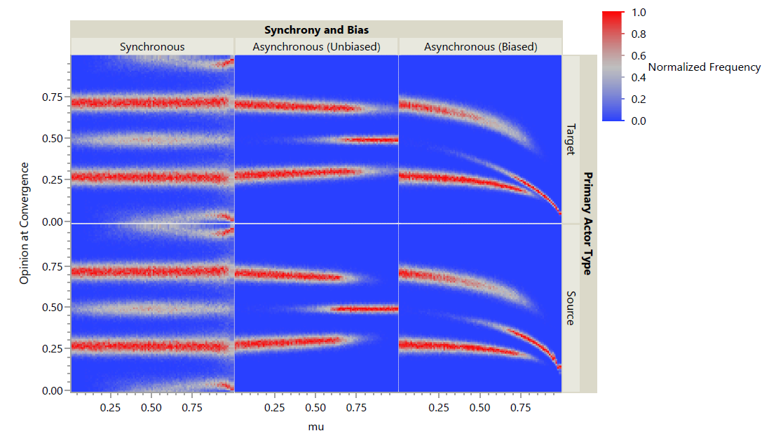
Normalized heat maps are shown in Figures 7 and 8. For these plots, the mean opinion within each cluster at convergence is treated as a separate outcome, regardless of how many agents were in that cluster. For each set of parameters (seen as a column within a plot), the associated histogram was constructed with bins of \(0.01\) and frequencies normalized such that a value of \(0\) is observed only if no outcome resulted in that opinion and a value of \(1\) is observed only if that opinion was the most frequently observed outcome for that set of parameters. Each dot in these plots is colored according to the normalized frequency, with red being the most common outcome and blue being unseen outcomes.
For \(s = 2\), all three primary actor types (target, source, group) were examined with and without synchrony. When schedules were asynchronous, both unbiased and biased forms were run. Figure 7 shows the results as a normalized heat map. This broad overview shows several interesting outcomes. As with the GRAM, source actors yield much higher variance in opinions in the model at convergence. Furthermore, as \(\mu\) increases for these schedules, the location of the most common clusters diverge toward the opinion poles. No obvious differences exist between schedules utilizing source actors with \(s=2\). For both target and group actors, there appears to be a difference in variance in cluster opinions in the synchronous and asynchronous schedules. Biasing effects appear mild for group actors but much stronger for target actors.
For \(s=\infty\), only source and target primary actors were simulated; as the action for group primary actors is defined, those models would be equivalent for both synchronous and asynchronous schedules. Furthermore, for synchronous schedules, source and target primary actors result in identical models; therefore, only target primary actors were simulated, although the results shown in Figure 8 show them in both positions for ease of comparison. While the GRAM showed the differences between schedules to be less drastic for \(s=\infty\), the GBCM shows the opposite trend. Synchronous schedules exhibit similar distributions of cluster opinions with \(s=\infty\) to those observed when \(s=2\). Asynchronous schedules, however, have no instances of extreme ''wings'' occurring across all values of \(\mu\) for either primary actor type, and only 9 observed instances of opinion convergence when \(\mu<0.25\). Instead, cluster opinions shift gradually toward a moderate opinion until they are near enough to converge when \(\mu\) is high. This pattern is observed for both unbiased and biased schedules, although ''moderate'' opinion is significantly affected by \(\mu\) for biased schedules for both actor types. It is also the opposite pattern to that observed for source actors when \(s=2\), in which clusters tended to diverge as \(\mu\) increased.
In order to compare the biasing effect across schedules, Figure 9 plots the mean opinion of all agents at convergence with the same parameters, regardless of cluster membership.
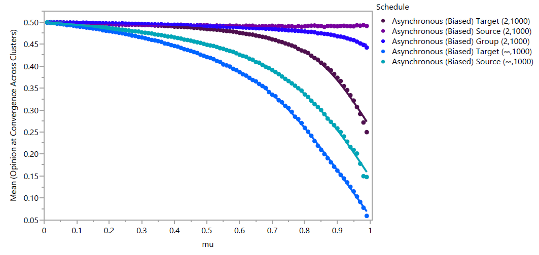
Unlike with GRAM, GBCM biasing effects have the same general pattern of increasing with respect to \(\mu\), allowing schedules to be rank-ordered by their biasing effect. As predicted, the Asynchronous Source \((2,1000)\) schedule exhibited the weakest biasing effect; mean opinion decreases by 0.0075 as \(\mu\) increases, which is visually imperceptible. From weakest to strongest, schedules are Asynchronous Source \((2,1000)\), Group \((2,1000)\), Target \((2,1000)\), Source \((\infty,1000)\), Target \((\infty,1000)\).
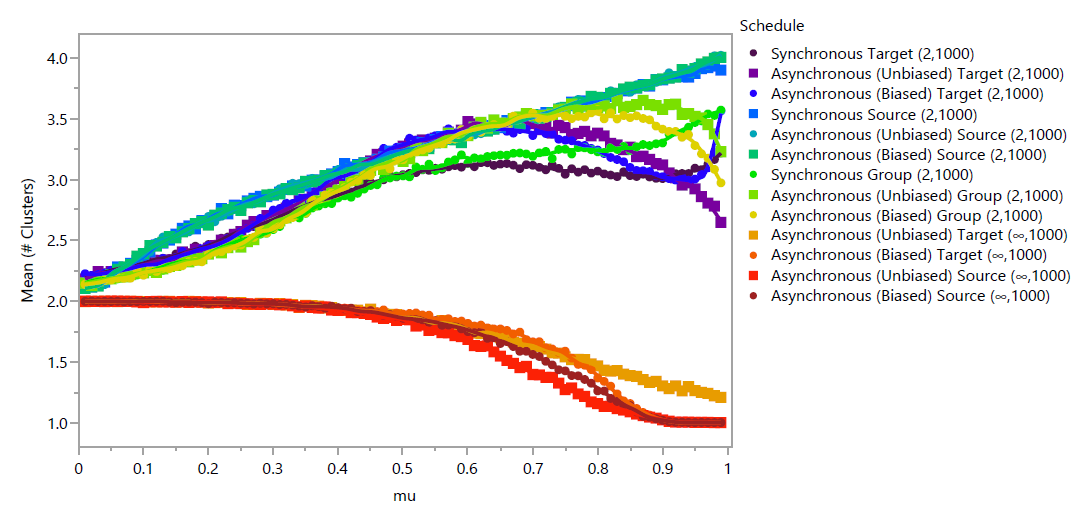
The feature that distinguishes bounded confidence models from repeated averaging models is the presence of distinct opinion clusters at convergence. As such, for these models, a primary measure of interest is the number of clusters that exist at convergence within a single replicate. Figure 10 shows the mean number of clusters of any size that exist for each schedule and \(\mu\) parameter across 1000 replicates. At low values of \(\mu\), all schedules result in approximately 2 clusters. When \(s=\infty\), the number of clusters decreases as \(\mu\) increases for all schedules. Of these, only the Asynchronous (Unbiased) Target \((\infty,1000)\) schedule does not reach a single cluster when \(\mu\) is sufficiently high. When \(s=2\), the number of clusters initially increases as \(\mu\) increases for all schedules. The number of clusters in the Synchronous Source \((2,1000)\), Asynchronous (Unbiased and Biased) Source \((2,1000)\), and Synchronous Group \((2,1000)\) schedules increase as a function of \(\mu\) across its entire range, while the function is non-monotonic for the remaining 5 schedules.
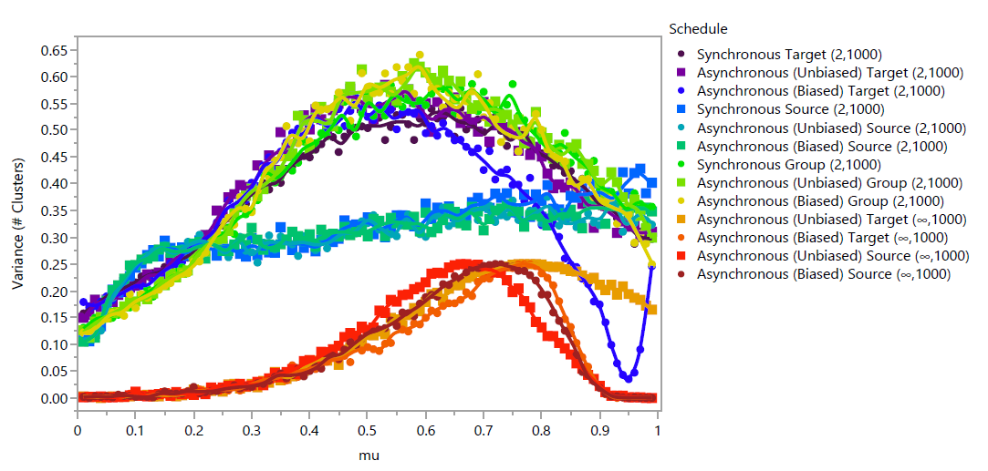
The variance in number of observed clusters between replicates, shown in Figure 11 also shows varying patterns for each schedule. For most schedules, the variance increases with \(\mu\) to a point, then decreases. The Asynchronous (Biased) Target \((2,1000)\) schedule is unique in resuming an increase at the highest values of \(\mu\), while the Synchronous and Asynchronous (Unbiased and Biased) Source \((2,1000)\) schedules stand out with variance that increases drastically up to \(\mu\approx 0.15\) and continuing to increase approximately linearly for the remaining range of \(\mu\).
Discussion
The most obvious qualitative observation for both the GRAM and GBCM is that varying the schedule of agent interactions can have significant impacts upon the emergent behavior observed. This is the primary intent of these models, and it suggests that schedules should be more clearly stated and justified in OD models. A clear and inclusive taxonomy such as SAS makes these discussions far easier.
In the GRAM, varying synchrony in all cases altered the relationship between the convergence parameter \(\mu\) and the variance in opinions observed at convergence. Varying the primary actor type had drastic effects upon that variance for \(s=2\), while that effect largely disappeared for \(s=\infty\).
In the GBCM, the patterns of where emergent clusters were located varied with synchrony, especially for high values of \(\mu\). For \(s=2\) and moderate values of \(\mu\), Asynchronous schedules were more likely to generate clusters toward the poles of the opinion spectrum (i.e., ''wings'') than synchronous schedules. For \(s=\infty\), only synchronous schedules ever resulted in these wings. The pattern of cluster locations was changed drastically by varying synchrony in this case. For all synchronous schedules, with sufficiently high values of \(\mu\), wings were more likely to be observed than clusters at more moderate locations; these models increasingly generated bi-polarization. For \(s=2\) and source-type primary actors, this effect was more clearly observed regardless of synchrony and bias; the most-observed clusters shifted toward the poles as \(\mu\) was increased.
The biased models were biased solely by the order in which agents were chosen to act. No schedule completely eliminated the effect of biased ordering, but in both models target actors were most affected by this ordering regardless of synchrony and parameters. This suggests that further research should be made into the dynamics of conversations; the assumption inherent to OD models that individuals speak with others in random order should be questioned. For example, it may be true that individuals tend to initiate conversations with like-minded others but are motivated to interject in existing conversations when they hear opinions that differ moderately from their own. This would imply a non-random order that may affect emergent behaviors.
There are social implications for each element of the agent schedule as well. Synchrony indicates whether individuals change their minds in the course of an interaction, or if their opinion shifts after the interaction is completed during a period of reflection. Scale parameters indicate the social activity levels of an individual by defining how many interactions they may have. This may vary by time, topic, and individual. Primary actor type reflects how an individual approaches interactions -- as a learner (target), as a teacher (source), or as a collaborator (group). An individual may have different motivations, and therefore different approaches, depending upon the situation. This mixture may also vary depending on the social status of that individual; writers for media outlets and individuals with many followers on social media may act as sources far more often than others.
An interesting and counter-intuitive outcome was observed in the GBCM with source actors for \(s=2\), where increasing the convergence parameter \(\mu\) increased the separation between the most observed clusters. The convergence parameter could alternatively be considered “susceptibility to influence,” as it is related to how much others’ opinions affect one’s own. This suggests that the presence of primarily source-type actors has a bi-polarizing influence. Partisan news sources and social media have been examined for their effects on bipolarization (see, for example, Levendusky 2013; Lee et al. 2014; Messing & Westwood 2014; Bakshy et al. 2015).
Conclusion
The SAS taxonomy represents a step toward creating a common language with which opinion dynamics researchers can compare models and discuss the social assumptions inherent to those schedules. This paper defines the taxonomy and examines variants of two generalized models using the mechanisms of repeated averaging and bounded confidence.
The outcomes of these models executed under various schedules show that varying any element of the schedule as defined can significantly affect emergent behavior in even relatively simple models. Existing models rely primarily upon randomization to order actions and choose agent type and synchrony without significant justification, but these can be interesting and useful inputs to a model. Furthermore, openly discussing these aspects of models can allow greater standardization and repeatability of models.
Model Documentation
The models were programmed using NetLogo 6.0 (Wilensky 1999) and the code is available at https://github.com/weimerc/GRAM-GBCM.References
ABELSON, R.P. (1964). ‘Mathematical models of the distribution of attitudes under controversy.’ In N. Frederiksen& L. L. Thurstone (Eds.), Contributions to Mathematical Psychology, (pp. 142–160). New York, NY: Holt, Rinehart, and Winston.
AXELROD, R. (1997). The dissemination of culture: A model with local convergence and global polarization. Journal of Conflict Resolution, 41(2), 203–226. [doi:10.1177/0022002797041002001]
AXELROD, R. & Tesfatsion, L. (2006). ‘Appendix AA guide for newcomers to agent-based modeling in the social sciences.’ In L. Tesfatsion, K.L. Judd (Eds.), Handbook of computational economics, Chapter 2, 1647-1659. [doi:10.1016/s1574-0021(05)02044-7]
BAKSHY, E., Messing, S. & Adamic, L. A. (2015). Exposure to ideologically diverse news and opinion on Facebook. Science, 348(6239), 1130–1132. [doi:10.1126/science.aaa1160]
BERGER, R. L. (1981). A necessary and sufficient condition for reaching a consensus using DeGroot’s method. Journal of the American Statistical Association, 76(374), 415. [doi:10.2307/2287844]
BONABEAU, E. (2002). Agent-based modeling: Methods and techniques for simulating human systems. Proceedings of the National Academy of Sciences, 99(Supplement 3), 7280–7287. [doi:10.1073/pnas.082080899]
BONNELL, T. R., Chapman, C. A. & Sengupta, R. (2016). Interaction between scale and scheduling choices in simulations of spatial agents. International Journal of Geographical Information Science, 30(10), 2075–2088. [doi:10.1080/13658816.2016.1158822]
BOURÉ, O., Fatès, N. & Chevrier, V. (2012). Probing robustness of cellular automata through variations of asynchronous updating. Natural Computing, 11(4), 553–564. [doi:10.1007/s11047-012-9340-y]
CARLEY, K. M. (1991). A theory of group stability. American Sociological Review, 56(3), 331–354. [doi:10.2307/2096108]
CARON-LORMIER, G., Humphry, R. W., Bohan, D. A., Hawes, C. & Thorbek, P. (2008). Asynchronous and synchronous updating in individual-based models. Ecological Modelling, 212(3-4), 522–527. [doi:10.1016/j.ecolmodel.2007.10.049]
CASTELLANO, C., Fortunato, S.& Loreto, V. (2009). Statistical physics of social dynamics. Reviews of Modern Physics, 81(2), 591–646. [doi:10.1103/revmodphys.81.591]
COLLINS, A., Petty, M., Vernon-Bido, D. & Sherfey, S. (2015). A Call to Arms: Standards for Agent-Based Modeling and Simulation. Journal of Artificial Societies and Social Simulation, 18(3), 12: https://www.jasss.org/18/3/12.html. [doi:10.18564/jasss.2838]
CORNFORTH, D., Green, D. G.& Newth, D. (2005). Ordered asynchronous processes in multi-agent systems. Physica D: Nonlinear Phenomena, 204(1-2), 70–82. [doi:10.1016/j.physd.2005.04.005]
DANDEKAR, P., Goel, A. & Lee, D. T. (2013). Biased assimilation, homophily, and the dynamics of polarization. Proceedings of the National Academy of Sciences of the United States of America, 110(15), 5791–5796. [doi:10.1073/pnas.1217220110]
DEFFUANT, G., Amblard, F., Weisbuch, G. & Faure, T. (2002). How can extremism prevail? A study based on the relative agreement interaction model. Journal of Artificial Societies and Social Simulation, 5(4), 1: https://www.jasss.org/5/4/1.html. [doi:10.18564/jasss.2211]
DEFFUANT, G., Neau, D., Amblard, F. & Weisbuch, G. (2000). Mixing beliefs among interacting agents. Advances in Complex Systems, 3(01n04), 87-98. [doi:10.1142/s0219525900000078]
DEGROOT, M. H. (1974). Reaching a consensus. Journal of the American Statistical Association, 69(345), 118–121. [doi:10.1080/01621459.1974.10480137]
DUGGINS, P. (2017). A psychologically-motivated model of opinion change with applications to American politics. Journal of Artificial Societies and Social Simulation, 20(1), 13: https://www.jasss.org/20/1/13.html. [doi:10.18564/jasss.3316]
EPSTEIN, J. M. (1999). Agent-based computational models and generative social science. Complexity, 4(5), 41–60. [doi:10.1002/(sici)1099-0526(199905/06)4:5<41::aid-cplx9>3.0.co;2-f]
EPSTEIN, J. M. (2006). Generative Social Science: Studies in Agent-Based Computational Modeling. Princeton: Princeton University Press. [doi:10.23943/princeton/9780691158884.003.0003]
EPSTEIN, J. M. & Axtell, R. (1996). Growing Artificial Societies: Social Science from the Bottom Up. Boston, MA: The MIT Press. [doi:10.7551/mitpress/3374.001.0001]
FATÈS, N. (2014). A guided tour of asynchronous cellular automata. Journal of Cellular Automata, 9(5-6), 387–416.
FATÈS, N. & Chevrier, V. (2010). Fatès, N., & Chevrier, V. (2010, May). How important are updating schemes in multi-agent systems? an illustration on a multi-turmite model. In Proceedings of the 9th International Conference on Autonomous Agents and Multiagent Systems: volume 1-Volume 1 (pp. 533-540). International Foundation for Autonomous Agents and Multiagent Systems.
FLACHE, A., Mäs, M., Feliciani, T., Chattoe-Brown, E., Deffuant, G., Huet, S., & Lorenz, J. (2017). Models of social influence: Towards the next frontiers. Journal of Artificial Societies and Social Simulation, 20(4), 2: https://www.jasss.org/20/4/2.html. [doi:10.18564/jasss.3521]
FRIEDKIN, N. E. (1999). Choice shift and group polarization. American Sociological Review, 64(6), 856–875. [doi:10.2307/2657407]
FRIEDKIN, N. E. (2001). Norm formation in social influence networks. Social Networks, 23(3), 167–189. [doi:10.1016/s0378-8733(01)00036-3]
GALAM, S. (1997). Rational group decision making: A random field Ising model at T= 0. Physica A: Statistical Mechanics and its Applications, 238(1-4), 66-80. [doi:10.1016/s0378-4371(96)00456-6]
GILBERT, N. & Troitzsch, K. (2005). Simulation for the Social Scientist. New York, NY: Open University Press.
GRIMM, V., Berger, U., DeAngelis, D. L., Polhill, J. G., Giske, J. & Railsback, S. F. (2010). The ODD protocol: A review and first update. Ecological Modelling, 221(23), 2760–2768. [doi:10.1016/j.ecolmodel.2010.08.019]
HARARY, F. (1959). A criterion for unanimity in French’s theory of social power. In D. Cartwright (Ed.), Studies in Social Power, (pp. 168–182). Ann Arbor, MI: University of Michigan.
HEGSELMANN, R. & Krause, U. (2002). Opinion dynamics and bounded confidence: Models, analysis and simulation. Journal of Artificial Societies and Social Simulation, 5(3), 2: https://www.jasss.org/5/3/2.html.
HOLLAND, J. H. (1995). Hidden Order: How Adaptation Builds Complexity (No. 003.7 H6).
HOLLEY, R. A. & Liggett, T. M. (1975). Ergodic theorems for weakly interacting infinite systems and the voter model. The Annals of Probability, 3(4), 643–663. [doi:10.1214/aop/1176996306]
JAGER, W. & Amblard, F. (2005). Uniformity, Bipolarization and Pluriformity Captured as Generic Stylized Behavior with an Agent-Based Simulation Model of Attitude Change. Computational & Mathematical Organization Theory, 10(4), 295–303. [doi:10.1007/s10588-005-6282-2]
LEE, J. K., Choi, J., Kim, C. & Kim, Y. (2014). Social media, network heterogeneity, and opinion polarization. Journal of Communication, 64(4), 702–722. [doi:10.1111/jcom.12077]
LEVENDUSKY, M. S. (2013). Why do partisan media polarize viewers? American Journal of Political Science, 57(3), 611–623. [doi:10.1111/ajps.12008]
LORENZ, J. (2010). Heterogeneous bounds of confidence: Meet, discuss and find consensus! Complexity, 15(4), 43–52. [doi:10.1002/cplx.20295]
MACAL, C. M. (2016). Everything you need to know about agent-based modelling and simulation. Journal of Simulation, 10(2), 144–156. [doi:10.1057/jos.2016.7]
MACAL, C. M. & North, M. J. (2014). Introductory tutorial: Agent-based modeling and simulation. In Proceedings of the 2014 Winter Simulation Conference, (pp. 6–20). IEEE. [doi:10.1109/wsc.2014.7019874]
MARK, N. (1998). Beyond individual differences: Social differentiation from first principles. American Sociological Review, 63(3), 309–330. [doi:10.2307/2657552]
MARTINS, A. C. R. (2009). Bayesian updating rules in continuous opinion dynamics models. Journal of Statistical Mechanics: Theory and Experiment, 2009(02), P02017. [doi:10.1088/1742-5468/2009/02/p02017]
MARTINS, A. C. R., Pereira, C. d. B.& Vicente, R. (2009). An opinion dynamics model for the diffusion of innovations. Physica A: Statistical Mechanics and its Applications, 388(15-16), 3225–3232. [doi:10.1016/j.physa.2009.04.007]
MÄS, M. & Flache, A. (2013). Differentiation without distancing: Explaining bi-polarization of opinions without negative influence. PLoS ONE, 8(11), e74516. [doi:10.1371/journal.pone.0074516]
MÄS, M., Flache, A. & Helbing, D. (2010). Individualization as driving force of clustering phenomena in humans. PLoS Computational Biology, 6(10), e1000959. [doi:10.1371/journal.pcbi.1000959]
MÄS, M., Flache, A. & Kitts, J. A. (2014). ‘Cultural integration and differentiation in groups and organizations.’ In V. Dignum and F. Dignum (Eds.) Perspectives on culture and agent-based simulations. Cham: Springer, pp. 71-90. [doi:10.1007/978-3-319-01952-9_5]
MÄS, M., Flache, A., Takács, K., & Jehn, K. A. (2013). In the short term we divide, in the long term we unite: Demographic crisscrossing and the effects of faultlines on subgroup polarization. Organization science, 24(3), 716-736. [doi:10.1287/orsc.1120.0767]
MESSING, S. & Westwood, S. J. (2014). Selective Exposure in the Age of Social Media. Communication Research, 41(8), 1042–1063. [doi:10.1177/0093650212466406]
NORTH, M. J. & Macal, C. M. (2007). Managing Business Complexity: Discovering Strategic Solutions with Agent-Based Modeling and Simulation. Oxford, MA: Oxford University Press.
NOWAK, A., Szamrej, J. & Latané, B. (1990). From private attitude to public opinion: A dynamic theory of social impact. Psychological Review, 97(3), 362–376. [doi:10.1037//0033-295x.97.3.362]
PAGE, S. E. (1997). On incentives and updating in agent based models. Computational Economics, 10(1), 67–87.
RAILSBACK, S. F. & Grimm, V. (2011). Agent-Based and Individual-Based Modeling: A Practical Introduction. Princeton, NJ: Princeton University Press.
SALZARULO, L. (2006). A continuous opinion dynamics model based on the principle of meta-contrast. Journal of Artificial Societies and Social Simulation, 9(1), 13: https://www.jasss.org/9/1/13.html.
SCHELLING, T. C. (1971). Dynamic models of segregation. The Journal of Mathematical Sociology, 1(2), 143–186.
SÎRBU, A., Loreto, V., Servedio, V. D., & Tria, F. (2017). ‘Opinion dynamics: models, extensions and external effects.’ In V. Loreto, M. Haklay, A. Hotho, V.D.P. Servedio, G. Stumme, J. Theunis, & F. Tria (Eds.), Participatory Sensing, Opinions and Collective Awareness. Cham: Springer, pp. 363-401. [doi:10.1007/978-3-319-25658-0_17]
STAUFFER, D., Sousa, A. O. & Moss de Oliveira, S. (2000). Generalization to square lattice of Sznajd sociophysics model. International Journal of Modern Physics C, 11(6), 1239–1245. [doi:10.1142/s012918310000105x]
SZNAJD-WERON, K. & Sznajd, J. (2000). Opinion evolution in closed community. International Journal of Modern Physics C, 11(6), 1157–1165. [doi:10.1142/s0129183100000936]
URBIG, D., Lorenz, J. & Herzberg, H. (2008). Opinion dynamics: The effect of the number of peers met at once. Journal of Artificial Societies and Social Simulation, 11(2), 4: https://www.jasss.org/11/2/4.html.
WEIMER, C.W., Miller, J. O. & Hill, R. R. (2016). Agent-based modeling: An introduction and primer. In Proceedings of the 2016 Winter Simulation Conference, (pp. 65–79). IEEE Press. [doi:10.1109/wsc.2016.7822080]
WILENSKY, U. (1999). Center for connected learning and computer-based modeling. In NetLogo. Northwestern University: http://ccl.northwestern.edu/netlogo/.
WILENSKY, U. & Rand, W. (2015). An Introduction to Agent-Based Modeling: Modeling Natural, Social, and Engineered Complex Systems with NetLogo. New York, NJ: The MIT Press.