
Introduction
Political polarization has increased steeply over recent years in many democratic societies, up to the point of posing a threat to political stability (Hare & Poole 2014; Abramowitz & Saunders 2008). If we want to explain the continuing surge of polarization, it is crucial to understand the psychological and social mechanisms that generate it, and the circumstances under which they operate. Polarization can be defined as "division into two conflicting or contrasting groups" (American Heritage Dictionary 2011). Political scientists stipulate two essential aspects of polarization: opinion extremeness (how far positions are from the center) and issue constraint (how positions on different issues correlate) (Converse 1964; Baldassarri & Gelman 2008). Our aim with this study is to identify a minimal set of mechanisms that can generate these two essential aspects.
So far, the literature on polarization has largely focused on opinion extremeness. Opinion extremeness is quantified by how much the distribution of positions on various policy issues (such as abortion, immigration, or cannabis legalization) is concentrated on both fringes of a policy dimension, as opposed to the center (Fiorina & Abrams 2008). The emergence of opinion extremeness poses a theoretical problem: Most psychological research on social influence has produced examples of assimilative influence, in which individuals’ opinions become more similar upon interaction (see Flache et al. 2017; Lorenz et al. 2011). But if social influence is only assimilative, it can be shown that all individuals in a society would sooner or later converge to a complete consensus on all issues (as long as they are at least indirectly connected; Abelson (1964); Berger (1981)). However, in reality we do not observe societies in a complete consensus state, suggesting that social influence cannot be exclusively assimilative. And indeed, several studies have found that social influence can also be repulsive, meaning interacting individuals become more dissimilar (Hovland et al. 1957; Cohen 1962; Nyhan & Reifler 2010; Bail et al. 2018). This phenomenon, also known as backfire effect, negative social influence or boomerang effect, is thought to occur between individuals whose opinions are already quite dissimilar. The existence of a backfire effect could explain how opinions diverge into opposite extremes. The problem is that there are also multiple studies which do not confirm the existence of a backfire effect (Takács et al. 2016; Wood & Porter 2019). So far, no explanation for this mixed evidence has been put forward.
While explaining opinion extremeness is an important problem, political scientists have stressed that extreme opinions are necessary, but not sufficient for a society to be polarized. Positions on different policy issues also need to be correlated with each other – a property known in political science as issue constraint (Converse 1964). Issue constraint has been observed empirically in populations at large (Baldassarri & Gelman 2008; DellaPosta et al. 2015), as well as in the outcomes of group discussions. Latané & Bourgeois (2001) showed how a limited social network structure can lead to issue constraint (correlation between opinion dimensions) when participants interact in a conformity game where there is an incentive to agree with one’s neighbors. In practice, low issue constraint means that the positions of political actors on any one issue are independent from their positions on other issues. Under low issue constraint, political actors can have any combination of issue positions and none of these combinations will be substantially more frequent than any other in the population. For political actors who want to form alliances, this poses a problem: They would rarely encounter other actors with whom they agree on many issues, as most actors would agree and disagree with each other on roughly half of all issues. This makes the formation of stable political alliances very difficult, since political actors who are, for example, jointly supporting cannabis legalization, will likely find themselves opposing each other on the next issue, for example abortion. Thus, without issue constraint, opinion extremeness alone does not constitute polarization, but political fragmentation.
In political systems with high issue constraint, a multitude of issue positions can be described by a position on a single ideological dimension with negligible loss of information. For example, instead of describing certain political actors as ’in favor of gun control, cannabis legalization, and against increased defense spending, etc.’, we can just describe them with the word ’leftist’. Most political systems are characterized by such an ideological dimension, usually labeled ’left-right’ or ’liberal-conservative’ (Benoit & Laver 2006). It has been shown that even many non-political issues, such as taste in music or belief in horoscopes, align to some degree with this ideological dimension (DellaPosta et al. 2015). Poole (2005) highlights the origin of opinion constraint as a major open research question in political science (see also Hare & Poole 2014). He notes that "this bundling [of issue dimensions] does not have to be a function of a logically consistent philosophy" (Poole 2005, p. 204). This means that often there is only a very distant, if any, logical connection between issue positions, such as gay marriage and corporate tax. Of course, one can always construct an ad hoc connection between two given issues, but finding a consistent principle that explains issue constraint is still an open question (DellaPosta et al. 2015). It remains to be tested whether issue constraint can emerge from the micro-level interactions between individuals without the need to assume a preexisting complex structure, such as logical links between issues (Schweitzer 2018).
To clarify that polarization is not just opinion extremeness, we define hyperpolarization as the coexistence of opinion extremeness and issue constraint in a multidimensional opinion space. By definition, a metric of hyperpolarization of a political system must be maximal if 1) the political system is divided into two blocks, each encompassing half of the population, 2) each of these two blocks has perfect internal consensus on all relevant issues, and 3) the blocks are in total disagreement with each other on all relevant issues (see also Flache & Macy 2011; Esteban & Ray 1994). By definition, a metric of hyperpolarization must be lower if there are more or less than two political blocks, if the size difference between blocks is large, if there is disagreement within blocks, or if there is agreement (at least on some issues) between different blocks. Consequently, hyperpolarization is zero if a political system is in a state of complete consensus on all relevant issues.
Our goal is to explain the emergence of hyperpolarization from the interactions between individuals without having to assume complex social or logical structures. To do so, we develop a theory of opinion change that, when formulated as a computational model, simultaneously generates both aspects of hyperpolarization: opinion extremeness and issue constraint. In Section 2, we give a brief overview of polarization models in the opinion dynamics literature, highlighting the models that generate some aspects of hyperpolarization. In Section 3, we present Weighted Balance Theory (WBT) , and empirically test some of its propositions against data from the American National Election Survey (ANES). In Section 4, we develop an opinion dynamics model based on WBT and our empirical analyses. We introduce a metric to quantify hyperpolarization from the multidimensional issue positions of agents, and apply this metric to show the hyperpolarization outcomes of our model under a wide range of circumstances.
Literature on Opinion Dynamics Models of Polarization
Opinion dynamics models typically encompass a number of agents characterized by issue positions on one or several, discrete or continuous opinion dimensions. These agents influence each other’s opinions over time, following specified rules of interaction that produce different opinion distributions.
One-dimensional opinion dynamics models
Most conventional opinion dynamics models have focused on the extremeness aspect of polarization (for reviews, see Lorenz 2007; Flache et al. 2017), and have treated the existence of a single ideological dimension as given, instead of as an emergent phenomenon in need of explanation. As described by Mäs & Flache (2013) and Flache et al. (2017), one-dimensional models of continuous opinions can be categorized into three classes:
- models with only positive influence between agents always create consensus (Abelson 1964; Berger 1981),
- bounded confidence models, in which agents only interact with similar others, can create multiple opinion clusters (Deffuant et al. 2000; Hegselmann et al. 2002; Groeber et al. 2009; Lorenz 2007), and
- models with repulsion between dissimilar agents can create bi-polarization (Jager & Amblard 2005; Salzarulo 2006).
Model classes 2 and 3 can, for certain parameter values, replicate the extremeness aspect of hyperpolarization. However, when extended to multidimensional opinion spaces, they do not generate the issue constraint necessary for hyperpolarization, as we show in Appendix A.
Multidimensional models of hyperpolarization
Only few opinion dynamics models operate in multidimensional opinion spaces. To our knowledge, three of these multidimensional opinion dynamics models generate a form of hyperpolarization under special conditions: Huet & Deffuant (2010) (see also Huet & Mathias 2018) propose a model with two opinion dimensions, in which the dynamics on the second dimension is determined by the state of the first dimension. If two agents are close together on the first dimension, they will attract each other on both dimensions. If they are far apart on the first dimension, they do not exchange opinions on the first dimension (i.e., bounded confidence), and move further apart on the second dimension (rejection). Under certain parameter configurations, the model produces a hyperpolarized state with two clusters in opposite corners of the opinion space, and a third cluster in the middle, and thus a high degree of issue constraint and an intermediate degree of opinion extremeness. This dependence between dimensions is a way to encode issue constraint, not an attempt to generate issue constraint from interaction between individuals.
Flache & Mäs (2008) present a multidimensional model containing both opinion and demographic dimensions. While agents’ issue positions are continuous and change over time, demographic attributes are binary and immutable. Agents’ distance in the combined opinion-demographic space determines whether they approach or repulse each other. This model can generate hyperpolarization if the demographic dimensions are highly correlated. While this outcome is certainly interesting, it means that hyperpolarization in this model is not generated by its mechanisms, but is induced by design through the correlation of demographic attributes. Without demographic attributes the model is reduced to a multidimensional repulsion model that does not generate hyperpolarization (see Appendix A).
Finally, Flache & Macy (2011) explore a multidimensional opinion dynamics model that combines attraction and repulsion mechanisms with a caveman social network structure with densely connected clusters. While this model is able to create an intermediate degree of hyperpolarization for two opinion dimensions, hyper-polarization declines rapidly when they add more than two opinion dimensions. Therefore, besides requiring complex social structures, this model does not reproduce hyperpolarization for a realistic number of opinion dimensions. To sum up, hyperpolarization has not been shown to emerge from standard modeling assumptions without additional social structures, like the caveman network, or correlated demographic dimensions from which issue constraint trivially follows.
Several of the models quoted in the last two sections are based on Social Identity Theory (SIT) (Huet & Deffuant 2010; Huet & Mathias 2018; Flache 2018), which justifies both assimilative social influence within social groups, and repulsive influence between groups (Tajfel et al. 1979; Turner et al. 1984; Brewer 1991). This might give rise to the expectation that SIT could explain the emergence of hyperpolarization. If we assume the existence of only two groups, this expectation is justified: If two groups repulse each other in a higher-dimensional opinion space, they will end up with diametrically opposed opinions, corresponding to maximal hyperpolarization. However, to our knowledge, SIT does not make any predictions about the number of groups arising in a given context. If there are more than two groups, we do not see any mechanism in SIT that would guarantee that these groups align to a major ideological dimension. And yet, this is largely the case in multi-party systems (Benoit & Laver 2006). In conclusion, the tenets of SIT do not seem to be sufficient to explain the emergence of hyperpolarization.
Weighted Balance Theory
Extending balance theory
The theory we present in this section is based on the assumption that the social influence an individual \(j\) exerts on another individual \(i\) is moderated by the interpersonal attitude of \(i\) towards \(j\) (i.e., to what degree \(i\) likes or dislikes \(j\)). In other words, our theory combines cognitive (issue positions) and affective components (interpersonal attitudes) to explain opinion change. We postulate that issue positions and interpersonal attitudes influence each other in a dynamic way: Interpersonal attitudes are influenced by issue positions – agreement fosters liking and disagreement fosters disliking. Conversely, issue positions are adapted to interpersonal attitudes – human beings want to agree with others they like and want to contradict who they dislike.
We formalize the rules of this mutual adaptation of issue positions and interpersonal attitudes in an extended version of Balance Theory, which we call Weighted Balance Theory (WBT). Balance Theory was developed by Heider (1946) to explain the cognitive organization of attitudes, and later expanded to social networks in the form of Structural Balance Theory by Cartwright & Harary (1956). According to Heider, attitudes can have positive or negative valence, and be directed to objects, ideas, events, or other individuals. Configurations of attitudes can be either balanced or imbalanced, and human beings strive to increase balance in their cognitive organization.
Heider specifically focuses on triads consisting of an ego \(i\), an alter \(j\), and an object \(d\). In the context of this paper, \(d\) is a particular policy issue. In the following, we will denote the attitude of an individual \(i\) to a political issue \(d\) as \(\mathbf{o}^i_d\), with \(\mathbf{o}^i\) being the opinion vector of individual \(i\), representing \(i\)'s attitudes towards all \(D\) policy issues under consideration. Each of these opinions has a sign, denoting whether the individual is in favor or against a certain issue. We denote the interpersonal attitude of \(i\) towards \(j\) as \(A_{ij}\). Note that \(\mathbf{o}^j_d\) is \(i\)'s perception of \(j\)'s attitude towards \(d\), and not necessarily the actual opinion of \(j\). Heider defines an \(i\)-\(j\)-\(d\) triad as in balance either if \(i\) has a positive attitude towards \(j\) and \(i\) and \(j\) agree in their attitudes towards \(d\) (i.e., their attitudes towards \(d\) have the same sign), or if \(i\) has a negative attitude towards \(j\) and they disagree about \(d\) (their attitudes have different signs). Generally speaking, an \(i\)-\(j\)-\(d\) triad is balanced if and only if the sign of each attitude relation is the product of the signs of the other two relations (Cartwright & Harary 1956).
Modeling attitudes as purely binary, i.e. either positive or negative, is an oversimplification. In reality, attitudes do not only have a sign, but also a certain strength or weight: One can be more or less in favor of or against something, or neutral towards it. We define this weight to be a real number between \(0\) and \(1\). Thus, signed and weighted attitude relations can be represented by a real number between \(-1\) and \(1\). The necessity of expanding balance theory by including attitude weights was already acknowledged by Cartwright & Harary (1956).
To extend Balance Theory to include weights, we require a rule to compute the weight and sign of relations between individuals (see also Wiest 1965; Feather 1964). Let us assume we have a perfectly balanced \(i\)-\(j\)-\(d\) triad with signed and weighted relations between the three elements. If we only know the signs and weights of two of the three relations in the triad, how can we determine the third relation? We postulate two basic requirements:
- if the weight of any of the first two attitude relations in a \(i\)-\(j\)-\(d\) triad is zero, the third relation must be zero as well, in order to obtain a balanced triad. In other words, if \(i\) does not care about \(d\) either way, \(i\) will also not care about \(j\)'s attitude towards \(d\), and \(i\)'s resulting attitude towards \(j\) will be neutral.
- the weight of the third attitude relation should be between the weights of the first two relations.
Simply taking the product of the weights would satisfy requirement 1, but not requirement 2: If both \(i\) and \(j\) have a positive attitude of weight \(0.5\) towards \(d\), the product rule would predict an attitude relation of just \(A_{ij} = 0.25\). Taking the arithmetic mean, on the other hand, would satisfy requirement 2, but not requirement 1. Thus, to determine the attitude weight, we instead use the geometric mean, i.e., the square root of the product. In combination with the product rule for the sign of the attitude relation, this gives us a function that we call signed geometric mean (SGM). In its general form, the signed geometric mean of \(n\) numbers \(x_1,...,x_n\) is defined as:
| $$\mathrm{SGM}(x_1,...,x_n) = \prod_{i=1}^{n} sign(x_i) \left (\prod_{i=1}^{n} |x_i| \right )^{\frac{1}{n}}$$ | (1) |
A weighted \(i\)-\(j\)-\(d\) triad is balanced if and only if each of the attitude relations it contains is the SGM of the other two attitude relations. Thus, we can now formalize balance as a continuous property bounded between \(0\) and \(1\), by computing how far a given \(i\)-\(j\)-\(d\) triad is from the balanced state:
| $$\mathrm{B}(\mathbf{o}^i_d,\mathbf{o}^j_d,A_{ij}) = 1 - \frac{1}{6}(|\mathbf{o}^i_d - SGM(\mathbf{o}^j_d,A_{ij})| + |\mathbf{o}^i_j - SGM(\mathbf{o}^i_d,A_{ij})| + |A_{ij} - SGM(\mathbf{o}^j_d,\mathbf{o}^i_d)|)$$ | (2) |
Determining interpersonal attitudes
If the attitudes of \(i\) and of \(j\) towards issue \(d\) are known, we can apply the SGM to \(\mathbf{o}^i_d\) and \(\mathbf{o}^j_d\), in order to determine the interpersonal attitude \(A_{ij}\). Figure 1a shows the interpersonal attitude \(A_{ij}\) resulting from the position of \(i\) and \(j\) on issue \(d\). As in classical balance theory, the relation between \(i\) and \(j\) is positive if their attitudes towards \(d\) have the same sign, and negative otherwise. The intensity of their positive or negative relation is proportional to the intensity of their attitudes towards \(d\).
To model polarization in multidimensional opinion spaces, we have to define \(A_{ij}\) for cases where \(i\) and \(j\) have attitudes towards many different issues. In a first step, for each issue \(d=1,...,D\), we compute a separate \(\mathrm{SGM}(\mathbf{o}^{i}_{d},\mathbf{o}^{j}_{d})\), to then combine them to determine \(A_{ij}\). As an initial approximation, we assume that each issue contributes equally to \(A_{ij}\). We choose this as a parsimonious assumption, as in practice some issues might have higher weight than others.
| $$\overline{\mathrm{SGM}}(i,j) = \frac{1}{D}\sum_{d=1}^{D} \mathrm{SGM}(\mathbf{o}^{i}_{d},\mathbf{o}^{j}_{d})$$ | (3) |
We calculate \(A_{ij}\) as the result of applying a monotonously increasing function \(f(x)\) to the arithmetic mean of the SGMs:
| $$A_{ij} = f\left(\overline{\mathrm{SGM}}(i,j)\right)$$ | (4) |
Figure 1b depicts the interpersonal attitude of \(i\) towards \(j\) based on their \(2D\) opinion vectors. The axes represent the two opinion dimensions, \(d_1\) and \(d_2\), and the green arrow represents the opinion vector of individual \(j\), which is set to \(\mathbf{o}^j = [1,1]\) for this example. The color encodes the interpersonal attitude \(A_{ij}\) that would result from \(j\) interacting with an individual \(i\) at this position in the issue space. For example, the deep blue color in the bottom left corner tells us that an individual \(i\) with \(\mathbf{o}^i = [-1,-1]\) would have interpersonal attitude of \(-1\) to \(j\).
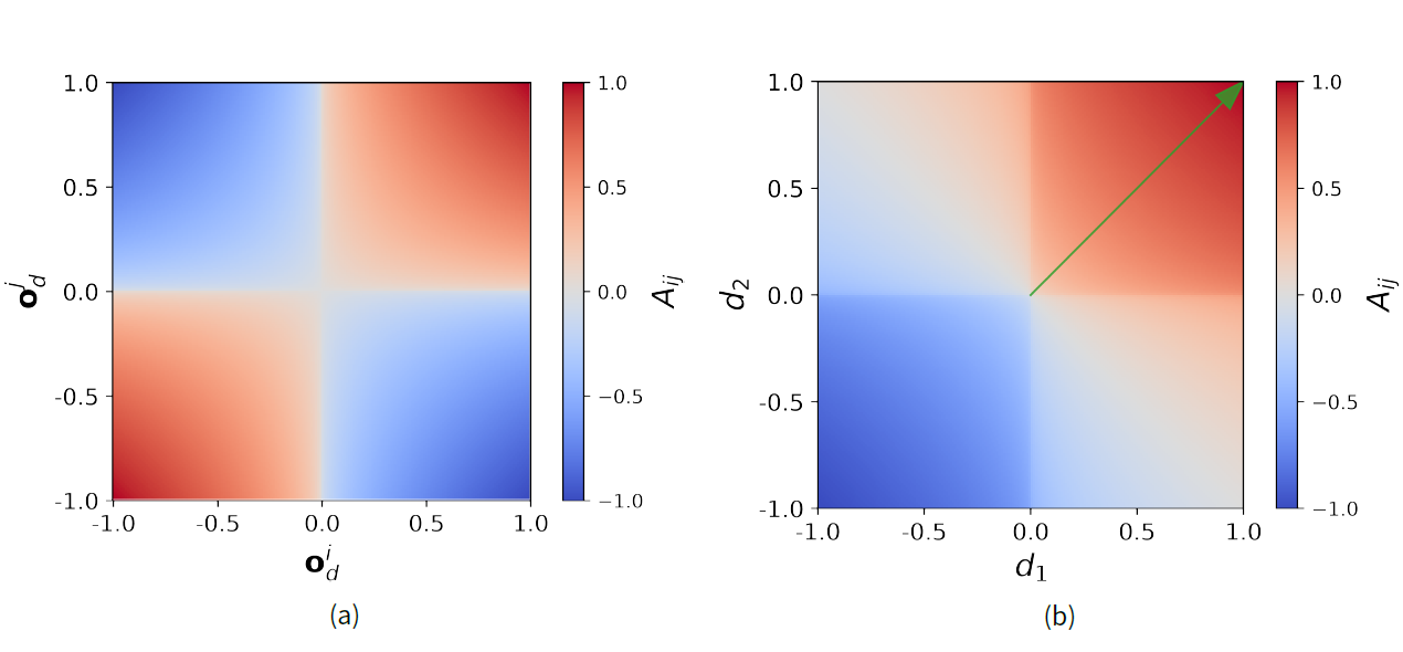
Figure 1b illustrates two interesting properties of the SGM: First, there is a sharp change in interpersonal attitude between the sectors of the coordinate system. This means that \(i\) is very sensitive to whether \(j\) is on the same side of all issues. And second, we can see that the transition between positive and negative interpersonal attitudes happens for vectors at a 90° angle from \(\mathbf{o}^i\). This generalizes to any other opinion vector, as well as to opinion spaces with more than two dimensions. The importance of being on the same side of an issue, as well as the relevance of the angle between opinion vectors, are major distinctive features between WBT and standard opinion dynamics models, which usually only take into account the distance between two agents on one or several opinion dimensions.
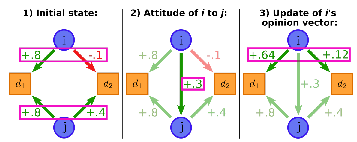
Balance maximization through opinion adjustment
Our next step is to show how opinion vectors change according to interpersonal attitudes, in order to increase balance (the complete process of opinion exchange is outlined in Figure 2). For example, if \(i\) has a positive attitude towards \(j\), but still disagrees with \(j\) on issue \(d\), the triangle \(i\)-\(j\)-\(d\) is imbalanced. To increase balance, \(i\) adapts its opinion on issue \(d\) to be in concordance with \(j\)'s opinion. The reverse is true if \(i\) dislikes \(j\): In this case, balance increases if \(i\) adapts its opinions in such a way as to increase the contradiction with \(j\). We can define an optimally balanced opinion vector \(\mathbf{b}^{ij}\), which represents the maximum of balance that \(i\) can achieve, given \(\mathbf{o}^j\) and \(A_{ij}\). This vector is generated by computing the signed geometric mean of \(A_{ij}\) with every component of \(\mathbf{o}^j\):
| $$\mathbf{b}_d^{ij} = \mathrm{SGM}(\mathbf{o}_d^j, A_{ij})$$ | (5) |
Heider’s central tenet is that individuals strive to increase the balance of their cognitive organization (Heider 1946). Given our definition of balance (Equation 2), increasing balance is equivalent to approaching the maximally balanced vector \(\mathbf{b}^{ij}\). However, it is reasonable to assume that opinions have a certain degree of inertia and do not change completely upon a single encounter with another person. Thus, we postulate that \(i\) does not reset its opinion vector \(\mathbf{o}^i\) completely to the balanced vector \(\mathbf{b}^{ij}\), but approaches \(\mathbf{b}^{ij}\) by a fraction \(\alpha\):
| $$\Delta \mathbf{o}_d^i = \alpha(\mathbf{b}_d^{ij} -\mathbf{o}_d^i )$$ | (6) |
The arrows of the quiver plot in Figure 3a depict the direction of opinion changes of an individual \(i\) when interacting with \(j\). Arrows are shown for several values of \(\mathbf{o}^i\) when interacting with a fixed opinion vector \(\mathbf{o}^j\) (green arrow). The background color shows the balance \(\mathrm{B}(\mathbf{o}^i,\mathbf{o}^j,A_{ij})\) between \(i\) and \(j\) before interacting (in our model setup, balance is always greater than \(0.5\), due to the fact that \(A_{ij}\) is computed to maximize balance). As we can see, if the angle between \(\mathbf{o}^i\) and \(\mathbf{o}^j\) is less than 90°, \(\mathbf{o}^i\) approaches \(\mathbf{o}^j\). Upon repeated interaction, \(\mathbf{o}^i\) would eventually converge to \(\mathbf{o}^j\). In contrast, if the angle between \(\mathbf{o}^i\) and \(\mathbf{o}^j\) is larger than 90°, \(\mathbf{o}^i\) would converge to \(-\mathbf{o}^j\).
WBT encodes the phenomenon of the backfire effect, which we discussed in the introduction section. A backfire effect occurs if an attempt to persuade an individual of a certain issue position produces the opposite result, i.e., the individual moves even further away from this position than before. In the opinion dynamics literature, the backfire effect is usually conceptualized as a function of the distance between two agents in opinion space (Flache et al. 2017): If two agents are more distant than a certain threshold value, they will repulse each other, i.e. become more distant after interaction (see Appendix A for simulations of this model). WBT offers an account of the backfire effect that differs from much of the opinion dynamics literature. In WBT, a backfire effect can occur, but only under certain conditions: First of all, the occurrence of a backfire effect is primarily determined by interpersonal attitudes, and not by issue positions. Issue positions are only relevant as far as they determine interpersonal attitudes. A negative interpersonal attitude is a necessary condition for the backfire effect.
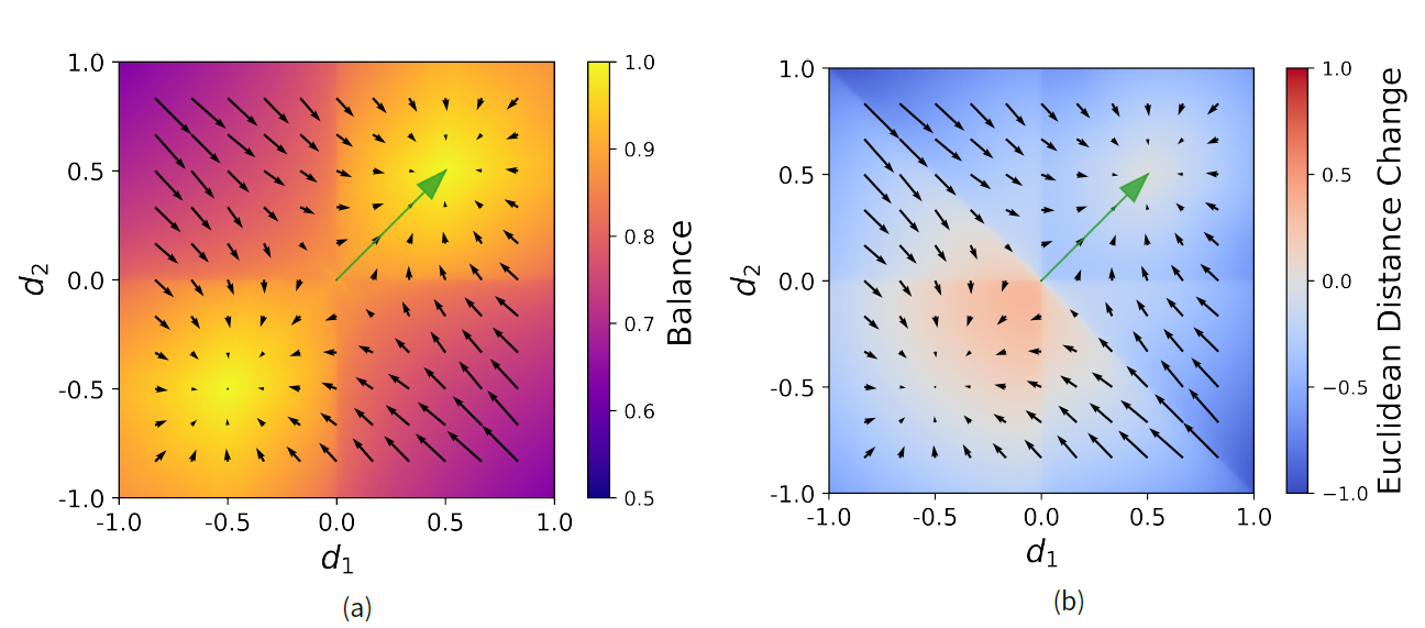
However, it is not a sufficient condition: As mentioned above, \(i\) will approach a maximally balanced vector \(\mathbf{b}^{ij}\), given by the SGM of the interpersonal attitude \(A_{ij}\) and \(j\)'s opinion vector \(\mathbf{o}^j\). A backfire effect will only occur if \(\mathbf{b}^{ij}\) is further away from \(\mathbf{o}^j\) than \(i\)'s current opinion vector \(\mathbf{o}^i\). In other words: The negative interpersonal attitude must be so strong that \(i\) feels that it still agrees too much with \(j\). If \(i\) disagrees with \(j\) to a degree that is congruent with their negative relation, there will be no backfire effect. Figure 3b shows the backfire effect in WBT with two opinion dimensions. As we can see, a backfire effect only occurs if \(\mathbf{o}^i\) and \(\mathbf{o}^j\) have a different sign in at least one dimension, and is strongest if they have different signs in both dimensions. But even in this case, the backfire effect only occurs if \(i\) is less extreme in its opinions than \(j\). Consequently, in WBT, repulsion and attraction are non-linear functions of distance in opinion space.
Empirical test of interpersonal attitude formation in weighted balance theory
WBT postulates that interpersonal attitudes are formed based on relative issue positions (Equation 4). In this section, we test this assumption and explore the shape of \(f(x)\) in survey data from the American National Election Study (ANES). ANES is a nationwide representative survey of American voters, conducted before and after every presidential election. Among other things, the 4270 respondents of the 2016 ANES survey were asked for their opinion on six different policy issues ranging from defense spending (increase vs decrease) to health insurance (government vs private) on 7-point rating scales. The respondents were also asked for their perception of the position of presidential candidates (Hillary Clinton and Donald Trump) on the same policy issues, again with 7-point scales. And finally, the respondents were asked to complete two affective thermometer scale items, on which they rated their subjective feelings towards each presidential candidate. These affective measures of attitudes towards candidates are measured with high resolution, from 0, meaning "very cold or unfavorable feeling" to 100, signifying "very warm or favorable feeling".
We rescale both the policy questions and the thermometer items between \(-1\) and \(1\), with \(0\) corresponding to a neutral position on the policy issues or a neutral attitude towards the presidential candidates. For every respondent, we construct:
- A 6-dimensional opinion vector \(\mathbf{o}^i\) of the respondent's own issue positions
- Two 6-dimensional opinion vectors of the respondent's perception of each presidential candidate's issue positions, \(\mathbf{o}^{i,Trump}\) and \(\mathbf{o}^{i,Clinton}\)
- The attitudes of the respondent towards each of the two presidential candidates, measured by the affective thermometer scales.
Due to respondents having missing values in at least one of the policy or thermometer items, our sample size is reduced to 2621 valid respondents for Hillary Clinton, and 2593 for Donald Trump. To predict each respondent's attitude towards each of the two presidential candidates, we apply Equation 4 to the respondent's own opinion vector \(\mathbf{o}^i\) and the respondent's estimates of the opinion vectors of the candidates, \(\mathbf{o}^{i,Trump}\) and \(\mathbf{o}^{i,Clinton}\), respectively.
The x-axes in Figure 4a show the average SGM between the positions of each respondent and each presidential candidate, whereas the y-axes represent the re-scaled thermometer ratings, separate for Hillary Clinton (left panel) and Donald Trump (right panel). The color encodes the logarithm of the number of respondents in each bin of a 2D histogram. If \(f(x)\) was the identity function, and we could perfectly predict the attitudes towards the presidential candidates, all respondents would lie on the diagonal. Clearly, this is not the case, but nevertheless the prediction with an identity function reaches \(R^2\) values of \(0.52\) for Clinton and \(0.46\) for Trump.
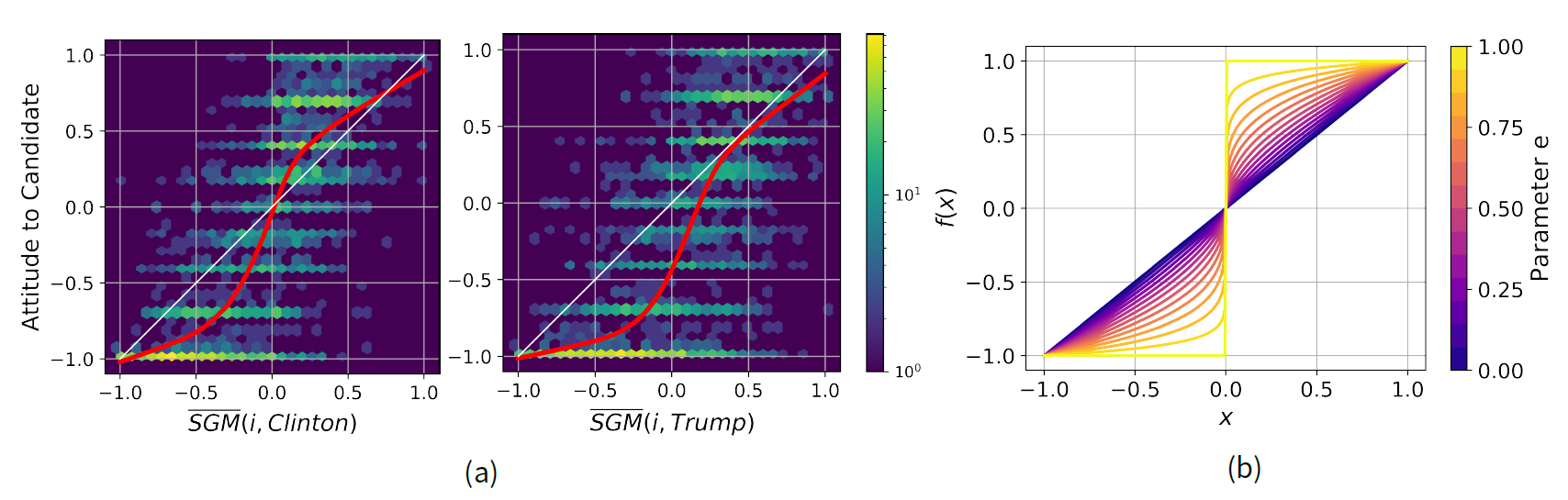
However, the thermometer ratings are not deviating from the WBT based predictions in a random fashion, i.e., towards both sides of the diagonal. The red curves in Figure 4a represent locally weighted regression (LOESS) curves. As we can see, for both candidates the LOESS curves have a sigmoid shape, a monotonically increasing form of \(f(x)\). For Hillary Clinton, if our prediction of the respondent’s attitude towards the presidential candidate is positive, the actual attitude tends to be even more positive. If the prediction is negative, the actual attitude tends to be even more negative. In other words, the thermometer ratings of Hillary Clinton tend to be on average more extreme than our predictions. For Donald Trump, the LOESS curve has a sigmoid shape too, only that it is below the diagonal. This probably reflects other, non-policy-related factors that cause respondents to judge him more negatively, and that are not captured by the ANES questionnaire.
Thus, in their judgment of political figures, respondents seem to tend to a ‘manichean’, black-and-white world view, in which "whoever is not with me is against me" (Matthew 12:30). We call this tendency evaluative extremeness. Further research will be necessary to determine whether evaluative extremeness is only present in the judgment of political figureheads like Clinton and Trump, or whether it is more widespread in social interactions (we discuss this further in Section 5). In the next Section, we describe how we implement evaluative extremeness in a WBT based opinion dynamics model. The degree of evaluative extremeness will play a crucial role for the behavior of this model.
Simulating Weighted Balance Theory
After describing the central tenets of Weighted Balance Theory, and empirically testing its predictions with regard to interpersonal attitudes, we now want to explore whether an opinion dynamics model based on WBT can generate hyperpolarization.
Notation and starting conditions
Every instance of our WBT opinion dynamics model (as well as the other models in the benchmark of Appendix A) contains \(N\) agents. The issue positions of each of these agents are represented by \(D\)-dimensional opinion vectors \(\mathbf{o}^{1},...,\mathbf{o}^{N}\). Each component represents the agent's attitude to a specific issue, quantified as a real number between \(-1\) and \(1\). When a new simulation starts, the components of every opinion vector of each agent are initiated uniformly at random. The simulation then proceeds in discrete time steps \(t=1,...,T\). The state of the model at time \(t\) can be characterized by a \(N \times D\) opinion matrix \(\mathbf{O}_t\), where the opinion vectors of all \(N\) agents are represented as row vectors.
At each time step \(t\), all \(N\) agents are selected in random order (thus, a single time step consists of \(N\) interactions). Each agent \(i\) then interacts with a randomly chosen other agent \(j\) and changes its opinion vector (asynchronous updating). These interaction pairs are chosen purely at random, without assuming any underlying social network or neighborhood structure (mean field approach; compare Groeber et al. 2014). We model interactions between agents as unilateral, meaning if agents \(i\) and \(j\) interact, agent \(i\) is influenced by \(j\), but not vice versa (of course, influence in the reverse direction can occur at another time). We run each simulation until it converges to a stable state. We assume a stable state is reached if, for five consecutive time steps, the changes in the opinion matrix are not larger than expected based on the noise level \(z\) (see following Section):
| $$|\mathbf{O}_t - \mathbf{O}_{t-1}| < D \cdot N \cdot z$$ | (7) |
Opinion exchange under evaluative extremeness
An interaction between two agents happens in three steps (see Figure 3): First, agent \(i\) determines its attitude towards agent \(j\), \(A_{ij}\), following Equation 4. Second, agent \(i\) adjusts its opinion vector \(\mathbf{o}^i\) to increase its balance with \(A_{ij}\) and \(\mathbf{o}^j\), following Equation 6. In the third step, every agent's opinion vector is affected by a noise vector in which each entry is independently drawn from a normal distribution with mean zero and standard deviation \(z\). This way, the parameter \(z\) controls the level of noise in the simulation. Adding certain amount of noise is important, since it has been found that, for bounded confidence models, polarized states that are stable in the absence of noise become unstable under low noise levels (Schweitzer & Hołyst 2000; Flache et al. 2017). The noise represents all influences not captured by the model, such as personal experiences and deliberations. By setting \(z>0\) and simulating the model several times, we ensure that our findings hold in realistic opinion dynamics scenarios affected by factors not covered by the model.
We implement evaluative extremeness in our model by changing the functional form of \(f(x)\) in Equation 4. First, we use the sigmoid LOESS curve retrieved from our analysis of the ANES data as functional form of \(f(x)\) (specifically the one for Hillary Clinton; see Section 3.22). We then develop a stylized version of this LOESS function, which is able to encode varying degrees of evaluative extremeness:
| $$f(x)= sign(x)\cdot|x|^{1-e}$$ | (8) |
Metrics
To quantify the different aspects of hyperpolarization, we will apply three different metrics to the opinion matrix \(\mathbf{O}\): A metric of opinion extremeness, \(E(\mathbf{O})\), a metric of issue constraint, \(C(\mathbf{O})\), and a direct metric of hyperpolarization, \(H(\mathbf{O})\), that we design to capture the coexistence of opinion extremeness and issue constraint.
First, we quantify the extremeness aspect of hyperpolarization, \(E(\mathbf{O})\), as the standard deviation of issue positions. If there is more than one issue dimension, we compute the arithmetic mean of the standard deviations on all different issue dimensions, i.e., the columns of the opinion matrix \(\mathbf{O}\). Second, we quantify issue constraint, \(C(\mathbf{O})\), as the average inter-correlation between opinion dimensions. More precisely, we compute Pearson correlations between all pairs of opinion dimensions, then apply the Fisher Z transformation to the absolute correlation values, and finally compute the arithmetic mean of the transformed values. In the last step, we back-transform this average into a correlation value by applying the inverse Fisher Z transformation. This average correlation is \(1\) if there is maximal issue constraint, and near zero if opinion values are completely independent. A high value of \(C(\mathbf{O})\) is a necessary condition for hyperpolarization but not a sufficient one: If all opinion vectors are distributed homogeneously along a diagonal through opinion space, issue constraint is maximal, but extremeness (and therefore hyperpolarization) is not.
And third, we design a metric to directly measure hyperpolarization, \(H(\mathbf{O})\), which takes into account both extremeness and constraint. If we compute all distances between unordered pairs of opinion vectors, it can be shown that the sum of these pairwise distances is maximal for the case of maximum polarization. Furthermore, if we square the pairwise distances between opinion vectors, their sum is uniquely maximal for the case of maximal polarization, i.e., there is no opinion matrix \(\mathbf{O}\) that is not maximally hyperpolarized and still reaches the maximal value of \(H(\mathbf{O})\). The metric takes the following form:
| $$H(\mathbf{O}) = \frac{1}{\delta^2_{max}} \frac{4}{N^2} \sum_{1=i<j}^{N} \delta(\mathbf{o}^i,\mathbf{o}^j)^2$$ | (9) |
\(H(\mathbf{O})\) is sensitive to the number of internally unanimous, mutually opposed factions in a political system, i.e., it decreases if the number of factions increases above two. \(H(\mathbf{O})\) is also sensitive to the relative size of these factions, meaning it decreases if one faction becomes bigger than the other. \(H(\mathbf{O})\) is zero if and only if there is complete consensus in a political system. This metric captures the definition of hyperpolarization we gave in the introduction, where the polarization of a political system is maximal if the population is split into two equal sized factions, who completely agree on all policy issues internally, but are maximally opposed to each other.
Simulation outcomes
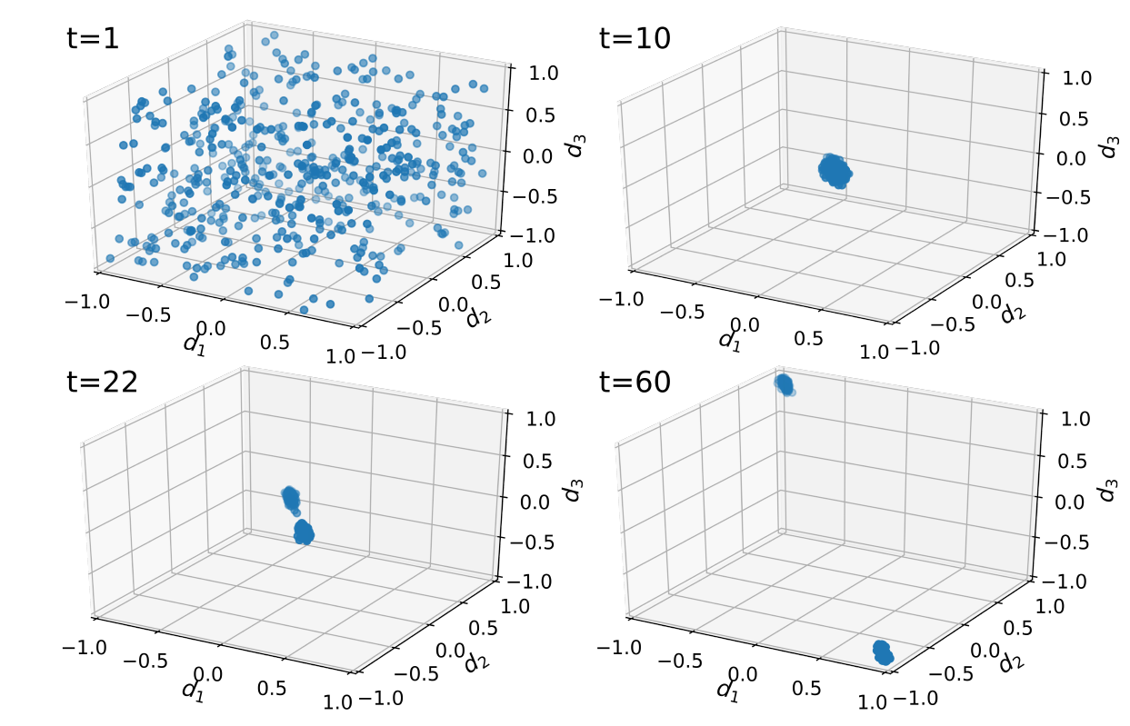
Figure 5 shows four snapshots of a simulation using the LOESS fit of attitudes towards Hillary Clinton as the functional form of \(f(x)\). This simulation was run with six issue dimensions, and a moderate noise level (\(z=0.01\)). The initial condition of a random distribution of opinions at \(t=1\) is followed by a transient state of consensus (\(t=10\)). However, as time evolves, two clusters of agents emerge and start separating from each other (\(t=22\)). At \(t=60\), these clusters come to rest in two opposite corners of the opinion space (Figure 5, lower right panel). This corresponds to a state of maximal hyperpolarization, with two maximally opposed political camps. This outcome proofs that our Weighted Balance Theory model can in fact produce a hyperpolarized state. Having demonstrated this, we want to further analyze the circumstances under which it produces hyperpolarization, and take a closer look at the model trajectory.
We analyze the conditions in which our WBT opinion dynamics model produces hyperpolarization in an exhaustive exploration for different values of the number of dimensions \(D\), the evaluative extremeness parameter \(e\), and the noise parameter \(z\). For all simulations, we set the number of agents in the system to \(N=500\), and the \(\alpha\)-parameter (controlling the speed of opinion change and the timescale of the model) to \(0.4\). All of these simulation runs under various parameter combinations converge to only two distinct states: Either a model run converges to a state of hyperpolarization, or to a state of consensus at the origin of the issue space. Figure 6a shows the median value of our hyperpolarization metric \(H\) in 100 simulations against the \(e\)-parameter value. If \(e = 0\), meaning if there is no evaluative extremeness, our model always converges to the consensus state (this is also true for \(e <0\), not shown here). Hyperpolarization can only emerge under evaluative extremeness (\(e > 0\)). In a model run without noise (\(z = 0\)), even a minimal degree of evaluative extremeness is enough to change the model outcome from consensus to maximal hyperpolarization, as illustrated by the abrupt jump of the blue lines in Figure 6a for \(e > 0\).
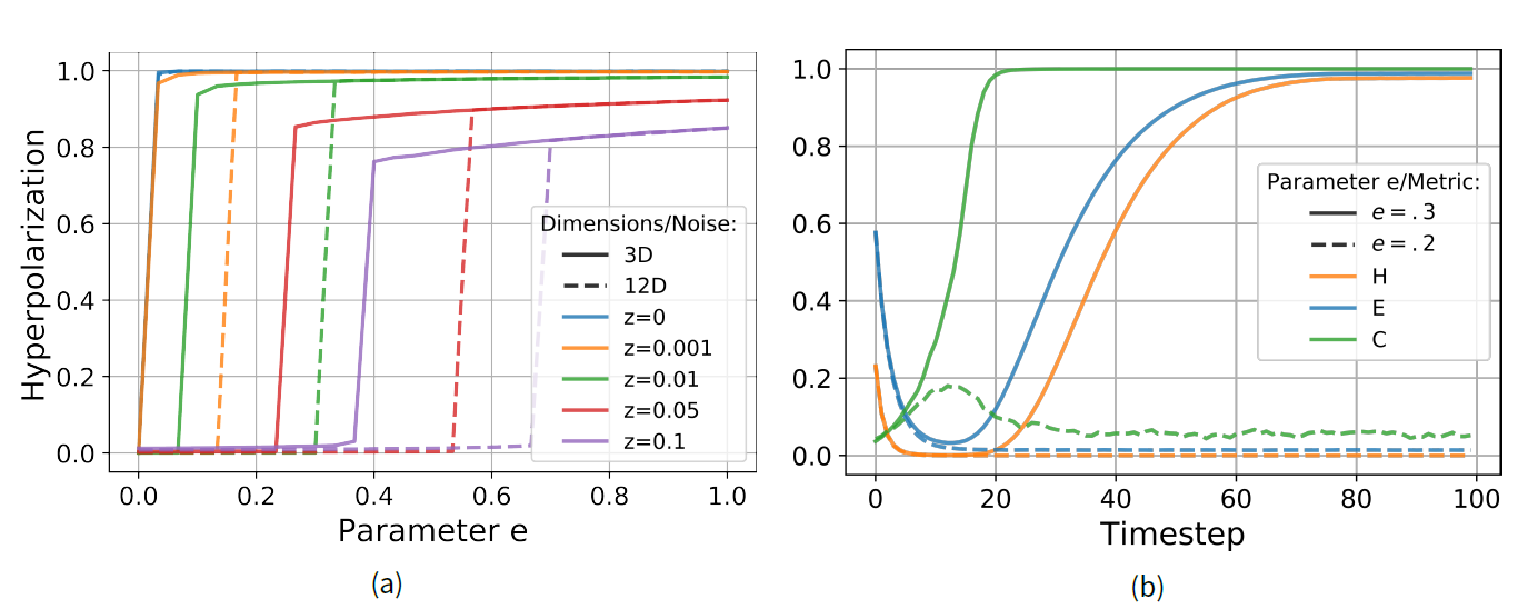
Higher noise levels \(z\) require higher values of \(e\) to generate hyperpolarization. For models with noise, increasing the number of opinion dimensions \(D\) has a similar effect: larger values of \(e\) are required to generate hyperpolarization for higher dimensionality \(D\). This can be seen in Figure 6a, where the hyperpolarization jumps in the dashed lines (\(D=12\)) are consistently to the right (higher \(e\)) of the solid lines (\(D=3\)). Thus, it seems that both noise and higher dimensionality hamper the emergence of hyperpolarization. A noiseless model, however, can generate hyperpolarization for arbitrary dimensionality. Interestingly, for some parameter combinations near the hyperpolarization jumps, both hyperpolarization and consensus can emerge, depending on random initial positions and sampling of agents.
Let us now look at two exemplary model runs, represented by the dashed and solid lines in Figure 6b. Both model runs have a dimensionality of \(D=12\) and a noise level of \(z=0.01\). They only differ in their degree of evaluative extremeness, which is \(e=0.2\) for the dashed line scenario, and \(e=0.3\) for the solid line scenario. As we can see from Figure 6a (dashed green line), these values of evaluative extremeness are on either side of the jump in hyperpolarization. Consequently, the model run with lower evaluative extremeness converges to a consensus state, whereas the model run with higher evaluative extremeness produces hyperpolarization.
While the end states of the two model runs are very distinct, their model trajectories initially look very similar: In both model runs, the extremeness of issue positions (\(E\)), as well as the hyperpolarization measure (\(H\)), go down steeply within the first ten time steps. At \(t=10\), the state of both model runs resembles the upper right panel in Figure 5: All agents are clustered around the center of the opinion space. The reason for this collapse becomes clear if we consider a simple geometrical principle: In higher-dimensional spaces, two random vectors are much more likely to be nearly orthogonal than either aligned or opposed (just like on earth, the equator region is more spacious than the polar regions). As Figure 1b illustrates, if two agents’ opinion vectors are orthogonal, they have a neutral interpersonal attitude towards each other. This neutral attitude renders every strong agreement or disagreement between agents on any issue dimension unbalanced. As we can see in Figure 2a, the consequence is a decrease in the magnitude of the opinion vectors, or in other words, a movement towards the origin of the issue space.
In both model runs, the initial decrease in extremeness is accompanied by an increase of issue constraint. This increase reflects a self-organization of the agents along a single diagonal of the opinion space – a nascent ideological dimension (which particular diagonal emerges as ideological dimension is random). Figure 1b illustrates the mechanism underlying this self-organization: Agents whose opinion vectors are at less than a 90° angle have a positive interpersonal relation. This motivates them to agree on even more issues, which in turn improves their relation, and so forth until the agents are perfectly aligned (see Figure 2a). The reverse happens if two agents are at an angle of more than 90°. Their negative relation will cause them to increase their disagreement, until their opinion vectors are diametrically opposed.
From \(t=10\), the trajectories of the two model runs diverge: For the dashed line model, the initial increase of issue constraint vanishes again, and from around \(t=30\) on, the model remains in a state low extremeness and negligible issue constraint. In contrast, issue constraint in the solid line model continues to rise until it reaches a maximum at \(t=20\). This increase of issue constraint triggers a rise of extremeness, and consequently, hyperpolarization. The crucial factor in this process is evaluative extremeness, which causes the agents to have more extreme interpersonal attitudes towards each other than warranted by their agreement or disagreement on the issues. This leads to a leap-frogging effect, in which agents strive to have more extreme opinions than their interaction partners, strongly resembling the social comparison effect promoted in group polarization theory (see Sunstein 2002). In this way, the agent population splits into two clusters around \(t=20\), which then migrate to two opposite corners of the issue space (see Figure 5, lower left panel). At \(t=70\), the system has reached a maximum of hyperpolarization, in which it remains indefinitely (see Figure 5, lower right panel). In the dashed line model, this self-reinforcing process is inhibited before it can even start: Due to the lower evaluative extremeness, the agents cannot overcome the disturbing effects of the noise. Thus, their issue constraint remains on a level below what is needed to initiate the process of hyperpolarization.
Discussion
In this article, we present an opinion dynamics model that, based on the psychological principles of WBT, simultaneously generates extreme opinions and issue constraint, the two aspects of hyperpolarization. To our knowledge, this is the first model that generates hyperpolarization without introducing complex social structures or preexisting demographic or opinion correlates. Different from other multidimensional opinion dynamics models, our WBT-based model generates hyperpolarization without introducing already hyperpolarized demographic dimensions (Flache & Mäs 2008), and without effectively reducing the dimensionality of the model by introducing issue constraint by design (Huet & Deffuant 2010). While complex network structures can generate hyperpolarization in low dimensional spaces (see Flache & Macy 2011), our model shows that there is no need to assume any particular network structure to generate hyperpolarization, even for cases with many opinion dimensions and random noise. However, this does not mean that network dynamics do not play a role in polarization dynamics, as previous models have shown the interplay between hierarchical network structures and opinion dynamics (Deffuant et al. 2013; Manzo & Baldassarri 2015; Hofstede et al. 2018). Future empirical research should focus on identifying how opinions and social networks influence each other in group experiments.
A decisive determinant of whether our model produces hyperpolarization or consensus is the degree of evaluative extremeness. Even in a model without noise, a minimal degree of evaluative extremeness is necessary to produce hyperpolarization. If this minimal degree of evaluative extremeness is present, however, our WBT based model produces maximal hyperpolarization for arbitrary numbers of opinion dimensions D. This appears as a first-order phase transition with a sharp jump between consensus and hyperpolarization for different values of e. We leave the analytical treatment of this phase transition for further research that can show whether it fits on a wider class of dynamical systems and to which extent it can lead to intermediate levels of polarization in the long run.
As the exemplary model runs in Figure 6b show, the trajectories of opinion extremeness and constraint are not parallel. Rather, opinion extremeness declines in the first part of the model run, while issue constraint rises. In the hyperpolarizing cases, opinion extremeness starts rising again once issue constraint has reached a high level. This poses a testable hypothesis: issue constraint starts to rise before opinion extremeness as part of the combination of balance dynamics and evaluative extremeness. Historical analyses using parliamentary or survey data could be used to test this prediction of the model.
The simulations of our model show the existence of a transient consensus state with low opinion extremeness but rising issue constraint, which eventually ends in hyperpolarization. This gives a new interpretation to the current growth of hyperpolarization across societies: perhaps the rules of opinion dynamics and information spreading have not changed so much, and we were on the road to hyperpolarization all along. Our model illustrates that there is no need for echo chambers to exist in order to generate hyperpolarization – it is enough to have cognitive balance dynamics with evaluative extremeness.
WBT encodes a formulation of the backfire effect in which the strength of the backfire is a nonlinear function of the distance between two individuals in opinion space. This nonlinearity could be one of the reasons why the backfire effect has not been found consistently across empirical studies (Hovland et al. 1957; Nyhan & Reifler 2010; Bail et al. 2018; Takács et al. 2016; Wood & Porter 2019). A second factor that could explain this discrepancy is based on non-political (positive and negative) influences on the quality of interpersonal attitudes. The fact that differences in political opinion do not always determine interpersonal attitudes might explain why the backfire effect does not reliably occur in empirical studies: For example, in a study where political arguments are supplied by the experimenter (Nyhan & Reifler 2010), it is quite unlikely that participants will dislike the experimenter just because they disagree with these arguments. Likewise, in a study where the issue under discussion is emotionally neutral (Mäs & Flache 2013), disagreement is unlikely to cause participants to develop negative attitudes towards each other. The lack of negative interpersonal attitudes might explain why these studies could not find a backfire effect. The situation in these studies is more likely to be governed by a general positivity bias, which we discuss in Appendix B. Thus, WBT proposes an interplay between interpersonal affect and opinion changes that has the potential to unify the current evidence on the backfire effect. The central role of interpersonal affect in WBT is supported by recent studies analyzing the emotional underpinnings of popular polarization in the US. Under the label of ’affective polarization’, researchers have shown how in the current political climate, even small differences in opinions are mapped into very negative feelings (Iyengar et al. 2012; Iyengar & Westwood 2015; Mason 2015b).
These outcomes also fit to our observation of evaluative extremeness in attitudes towards US presidential candidates. Our simulations reveal that the degree of evaluative extremeness is key to the emergence of polarization. This of course points us to the question where evaluative extremeness originates from. The psychological literature offers three mechanisms that increase evaluative extremeness: First, it has been found that emotional arousal induces a tendency towards more extreme evaluations (Clark et al. 1983, 1984). Thus, factors that induce more arousal, especially if they are related to political information, should contribute to increasing polarization. We do not have to look far for potential sources of arousal: The rise of ‘infotainment’ over the last decades has turned the induction of emotions from a side effect into the main objective of television news programs (Thussu 2008). One possible line of inquiry would be to enrich our model with a direct representation of affective dynamics (such as Schweitzer, Krivachy & Garcia 2020).
Second, research in social identity and self-categorization theory has revealed a tendency to evaluate groups more extremely than individuals (Sears 1983), as well as a tendency to increase the contrast between one’s ingroup identity and the identity of competing outgroups (Turner et al. 1984). Thus, increasing identification with political parties could explain a rise in evaluative extremeness. This is in line with studies showing a growing tendency towards tribalistic party identification in the US (Mason 2015a, b). However, so far little is known about the root causes of this tendency.
And third, evaluative extremeness also bears resemblance to the concept of ego involvement in Social Judgment Theory which reflects the subjective centrality of a given issue, and determines whether the issue "arouses an intense attitude", in contrast to a more detached factual treatment (Sherif & Hovland 1961, p. 191). Different from our concept of evaluative extremeness, however, high ego involvement does not just increase the intensity of attitudes, but also broadens the ‘latitude of rejection’, i.e., causes an individual to reject even relatively similar propositions. Whichever of these theoretical accounts we invoke, we have good reason to assume that evaluative extremeness is widespread in the political context, where emotional arousal, identification with groups, and ego-involvement are prevalent.
Conclusion
Explaining the emergence of opinion extremeness and issue constraint has long been a challenge to theorists in political science and opinion dynamics. In this article, we present a solution based on an extended version of Heider’s cognitive balance theory (Heider 1946), which we call Weighted Balance Theory. In contrast to other, more cognition-focused theories, WBT recognizes the importance of social emotions in explaining opinion dynamics. Whether two individuals’ opinions become more similar or dissimilar though interaction is determined by whether they like or dislike each other. But adapting their opinions can in turn change individuals’ interpersonal attitudes. Thus, in WBT, opinion change happens as a coevolution of interpersonal attitudes and opinions.
WBT explains 1) how individuals form weighted attitude relations towards each other based on their opinions on a variety of issues, and 2) how individuals increase the balance between their opinions and their interpersonal attitudes by adjusting the former to the latter. The driving force behind this coevolution is the need to reduce cognitive imbalance, which occurs when opinions and interpersonal attitudes are in conflict with each other, i.e., when individuals disagree with others they like, or agree with others they dislike.
We tested the first part of this theory, the relation between opinions and interpersonal attitudes, on data from the 2016 ANES survey. The results indicate that WBT can predict respondents’ attitudes towards two presidential candidates very well, but that these attitudes tend to be more extreme than our predictions. At least in a political setting, there seems to be a tendency towards a black-and-white world view. We call this tendency evaluative extremeness and implement it in the form of a sigmoid reweighing function into a WBT-based opinion dynamics model. We show that this model can reproduce hyperpolarization, as long as a minimal degree of evaluative extremeness is present. Furthermore, it can do this for an arbitrary number of dimensions, and under a considerable degree of random noise. Thus, WBT can explain the emergence of hyperpolarization in a robust and stable way.
WBT also gives us a new interpretation of the so-called backfire effect, in the modeling literature also known as repulsion (Jager & Amblard 2005; Salzarulo 2006). The standard description of the backfire effect is that individuals with very dissimilar opinions move further away from each other when they interact, rather than approaching a consensus position. WBT suggests a different interpretation of the backfire effect: Under WBT, individuals’ opinions only diverge if they dislike each other, and if their opinions are not different enough to be in balance with their negative interpersonal attitude.
In conclusion, WBT can offer a new perspective on the emergence of hyperpolarization, while at the same time integrating research strains from psychology, political science and opinion dynamics into an overarching theoretical framework.
Model Documentation
The model has been built in Phyton. The code to replicate our model is stored on the CoMSES Computational Model Library under the following url: https://www.comses.net/codebases/789bfc4e-a645-4b05-91f1-b91260e3576e/releases/1.0.0/.Acknowledgements
This research has been funded by the Vienna Science and Technology Fund (WWTF) through project VRG16-005.Appendix
A: Higher Dimensional Models of Attraction, Bounded Confidence and Repulsion
In this Appendix Section, we explore how the three mechanisms described in Section 2.2 (attraction, bounded confidence, and repulsion) behave in higher dimensions. In particular, we want to find out whether bounded confidence and repulsion can generate hyperpolarized opinion distributions.
Attraction: We model the attraction mechanism as a direct approach in multidimensional Euclidean space:| $$\Delta \mathbf{o}^i = \alpha(\mathbf{o}^j -\mathbf{o}^i ) + \mathbf{z}$$ | (10) |
Bounded confidence: We implement a multidimensional bounded confidence model by adding a threshold mechanism to the attraction model:
| $$\Delta \mathbf{o}^i = \Theta(e - \delta(\mathbf{o}^i, \mathbf{o}^j)) \cdot \alpha(\mathbf{o}^j -\mathbf{o}^i ) + \mathbf{z}$$ | (11) |
Repulsion: Lastly, we implement a multidimensional repulsion model by replacing the threshold mechanism from the bounded confidence model with a term that, beyond a certain distance threshold epsilon, changes attraction into repulsion:
| $$\Delta \mathbf{o}^i = (e - \delta(\mathbf{o}^i, \mathbf{o}^j)) \cdot \alpha(\mathbf{o}^j -\mathbf{o}^i ) + \mathbf{z}$$ | (12) |
The repulsion mechanism can cause opinion vectors to leave the bounds of the opinion space. To prevent this, opinion vectors have to be confined artificially to the interval \([-1,1]\).
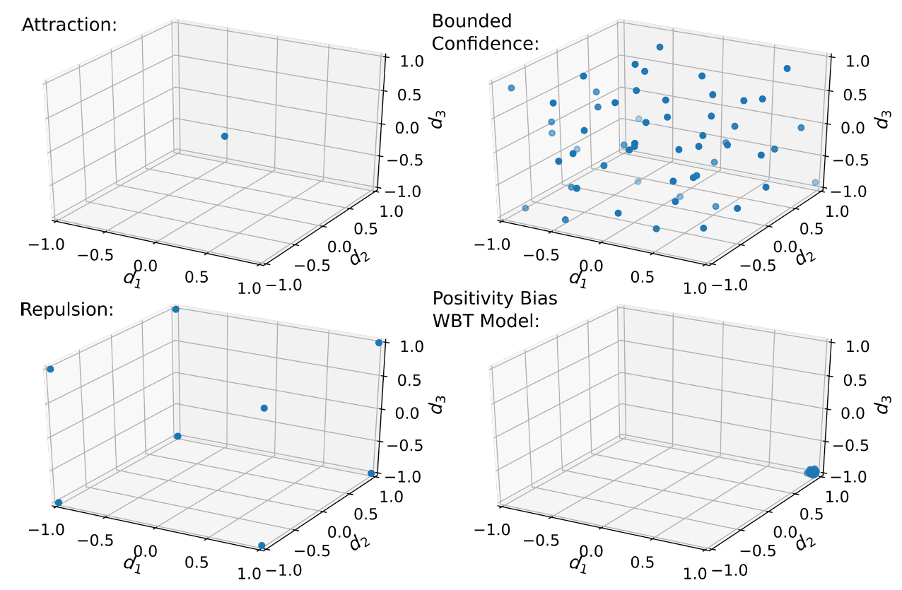
Even so, however, the repulsion model does not produce hyperpolarization. Depending on the value of \(e\), the model either converges to complete consensus near the center of the opinion space, or to a state of political fragmentation, as illustrated in Figure 7 (bottom left panel). In this state, the agents’ opinion vectors populate all corners of the opinion space in more or less equal numbers. While opinions in this state are maximally extreme, issue constraint is practically zero.
In conclusion, implementing standard opinion dynamics mechanisms in multidimensional spaces does not produce hyperpolarization, but either consensus or opinion fragmentation.
B: A Weighted Balance Model of Mono-Polarization
While some degree of hyperpolarization seems to be universal in societies at large, this is not the case in smaller social units, such as court juries, management teams, or church groups. When these social units deliberate an issue, they usually do not fission into two opposed groups, but instead converge to a consensus position. This consensus, however, tends to be more extreme than the mean of all initial positions – sometimes even more extreme than the most extreme initial position (Myers & Lamm 1975; Sunstein 2002).
Unfortunately, while qualitatively very different from hyperpolarization, this phenomenon has been dubbed ’group polarization’. To better distinguish the two phenomena, we call group polarization mono-polarization.
We quantify mono-polarization, \(M(\mathbf{O})\), as the sum of the dot products between all pairs of opinion vectors, normalized between \(0\) and \(1\):
| $$M(\mathbf{O}) = \frac{1}{D} \frac{2}{N(N-1)} \sum_{1=i<j}^{N} \mathbf{o}^i \cdot \mathbf{o}^j$$ | (13) |
The existence of mono-polarization poses a further challenge to theories of polarization: If deliberating groups usually come to an (extreme) consensus, why does this not happen in societies at large? Any theory of political polarization should also be able to explain this apparent discrepancy. In this section, we show that WBT can also account for mono-polarization.
Based on our empirical results in Section 3, we have assumed that individuals have a tendency towards evaluative extremeness. We implemented this tendency into our opinion dynamics model, and could show that it plays a crucial role in the emergence of polarization. However, there is reason to assume that evaluative extremeness is not universal in social relationships. Most social settings seem to be dominated by a bias towards positive evaluations of other individuals. For example, it has been found that employees expect to have positive relations with co-workers, and are strongly irritated by negative relations (Venkataramani et al. 2013). This preference for positive relations is part of a wider phenomenon called ’Pollyanna Principle’, which describes a preference for positive content in memory, cognition, and language (Boucher & Osgood 1969; Matlin & Stang 1978). Interestingly, it has been shown that positive relations among group members increase the strength of the mono-polarization effect (Brandstätter 1978; Sunstein 2002).
We implement this positivity bias into our model by replacing the functional form of \(f(x)\) in Equation 4. Instead of the identity function or the evaluative extremeness function (Equation 8), we use the following equation:
| $$f(x) = 2 \left ( \frac{x + 1}{2} \right )^{1-p} - 1$$ | (14) |
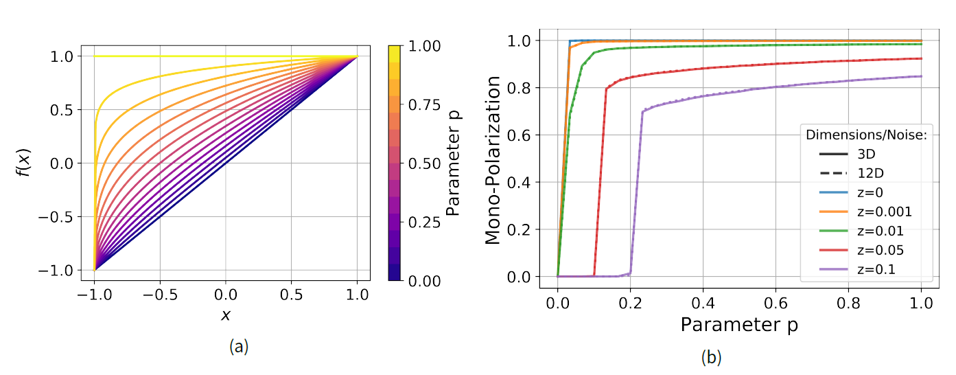
Once we implement the positivity bias in our model, it ceases to generate hyperpolarized opinion configurations. Instead, we obtain mono-polarization: All opinion vectors end up in a single corner of the opinion space, reflecting a maximally extreme consensus position (see Figure 7, bottom right panel). Figure 8b shows the degree of mono-polarization produced by simulation runs with varying positivity bias \(p\). If the positivity bias \(p\) is strong enough in relation to the noise level, the model produces maximal mono-polarization. Different from the case of hyperpolarization, this seems to be independent from the number of issue dimensions in the model.
In conclusion, a slight tweak of our WBT based model changes its dynamics radically: Instead of fissioning into two opposed clusters, agents now converge to a consensus, and then move together towards more and more extreme positions – reflecting the phenomenon of group mono-polarization. This demonstrates that, based on empirically plausible changes in the underlying mechanism, WBT can replicate qualitatively very different empirical phenomena.
References
ABELSON, R. (1964). ‘Mathematical models of the distribution of attitudes under controversy.’ In N. Fredericksen & H. Gullicksen (Eds.), Contributions to Mathematical Psychology. Holt, Rinehart & Winston.
ABRAMOWITZ, A. I. & Saunders, K. L. (2008). Is polarization a myth? The Journal of Politics, 70(2), 542–555.
AMERICAN HERITAGE DICTIONARY (2011). The American Heritage Dictionary: https://www.ahdictionary.com.
BAIL, C. A., Argyle, L. P., Brown, T. W., Bumpus, J. P., Chen, H., Hunzaker, M. F., Lee, J., Mann, M., Merhout, F. & Volfovsky, A. (2018). Exposure to opposing views on social media can increase political polarization. Proceedings of the National Academy of Sciences, 115(37), 9216–9221. [doi:10.1073/pnas.1804840115]
BALDASSARRI, D. & Gelman, A. (2008). Partisans without constraint: Political polarization and trends in American public opinion. American Journal of Sociology, 114(2), 408–446. [doi:10.1086/590649]
BENOIT, K. & Laver, M. (2006). Party Policy in Modern Democracies. London: Routledge.
BERGER, R. L. (1981). A necessary and sufficient condition for reaching a consensus using Degroot’s method. Journal of the American Statistical Association, 76(374), 415–418. [doi:10.1080/01621459.1981.10477662]
BOUCHER, J. & Osgood, C. E. (1969). The Pollyanna hypothesis. Journal of Verbal Learning and Verbal Behavior, 8(1), 1–8. [doi:10.1016/s0022-5371(69)80002-2]
BRANDSTÄTTER, H. (1978). ‘Social emotions in discussion groups.’ In H. Brandstätter, J. H. Davis & H. Schuler (Eds.), Dynamics of Group Decisions, chap. 6, (pp. 93–111). London: Sage Publications.
BREWER, M. B. (1991). The social self: On being the same and different at the same time. Personality and Social Psychology Bulletin, 17(5), 475–482. [doi:10.1177/0146167291175001]
CARTWRIGHT, D. & Harary, F. (1956). Structural balance: A generalization of Heider’s theory. Psychological Review, 63(5), 277. [doi:10.1037/h0046049]
CLARK, M. S., Milberg, S. & Erber, R. (1984). Effects of arousal on judgments of others’ emotions. Journal of Personality and Social Psychology, 46(3), 551. [doi:10.1037/0022-3514.46.3.551]
CLARK, M. S., Milberg, S. & Ross, J. (1983). Arousal cues arousal-related material in memory: Implications for understanding effects of mood on memory. Journal of Verbal Learning and Verbal Behavior, 22(6), 633–649. [doi:10.1016/s0022-5371(83)90375-4]
COHEN, A. R. (1962). A dissonance analysis of the boomerang effect. Journal of Personality.
CONVERSE, P. E. (1964). The nature of belief systems in mass publics (1964). Critical Review, 18(1-3), 1–74. [doi:10.1080/08913810608443650]
DEFFUANT, G., Carletti, T. & Huet, S. (2013). The Leviathan model: Absolute dominance, generalised distrust, small worlds and other patterns emerging from combining vanity with opinion propagation. Journal of Artificial Societies and Social Simulation, 16(1), 5: https://www.jasss.org/16/1/5.html. [doi:10.18564/jasss.2070]
DEFFUANT, G., Neau, D., Amblard, F. & Weisbuch, G. (2000). Mixing beliefs among interacting agents. Advances in Complex Systems, 3(01n04), 87–98. [doi:10.1142/s0219525900000078]
DELLAPOSTA, D., Shi, Y. & Macy, M. (2015). Why do liberals drink lattes? American Journal of Sociology, 120(5), 1473–1511. [doi:10.1086/681254]
ESTEBAN, J. M. & Ray, D. (1994). On the measurement of polarization. Econometrica: Journal of the Econometric Society, (pp. 819–851).
FEATHER, N. T. (1964). A structural balance model of communication effect. Psychological Review, 71(4), 291. [doi:10.1037/h0040059]
FIORINA, M. P. & Abrams, S. J. (2008). Political polarization in the American public. Annual Review of Political Science, 11, 563– 588 [doi:10.1146/annurev.polisci.11.053106.153836]
FLACHE, A. (2018). About renegades and outgroup haters: Modeling the link between social influence and inter-group attitudes. Advances in Complex Systems, 21(06n07), 1850017. [doi:10.1142/s0219525918500170]
FLACHE, A. & Macy, M. W. (2011). Small worlds and cultural polarization. The Journal of Mathematical Sociology, 35(1-3), 146–176 [doi:10.1080/0022250x.2010.532261]
FLACHE, A. & Mäs, M. (2008). Why do faultlines matter? A computational model of how strong demographic faultlines undermine team cohesion. Simulation Modelling Practice and Theory, 16(2), 175–191. [doi:10.1016/j.simpat.2007.11.020]
FLACHE, A., Mäs, M., Feliciani, T., Chattoe-Brown, E., Deffuant, G., Huet, S. & Lorenz, J. (2017). Models of social influence: Towards the next frontiers. Journal of Artificial Societies and Social Simulation, 20(4), 2: https://www.jasss.org/20/4/2.html. [doi:10.18564/jasss.3521]
GROEBER, P., Lorenz, J. & Schweitzer, F. (2014). Dissonance minimization as a microfoundation of social influence in models of opinion formation. The Journal of Mathematical Sociology, 38(3), 147–174. [doi:10.1080/0022250x.2012.724486]
GROEBER, P., Schweitzer, F. & Press, K. (2009). How groups can foster consensus: The case of local cultures. Journal of Artificial Societies and Social Simulation, 12(2), 4: https://www.jasss.org/12/2/4.html.
HARE, C. & Poole, K. T. (2014). The Polarization of Contemporary American Politics. Polity, 46(3), 411-429. [doi:10.1057/pol.2014.10]
HEGSELMANN, R., Krause, U. et al. (2002). Opinion dynamics and bounded confidence models, analysis, and simulation. Journal of artificial societies and social simulation, 5(3), 2: https://www.jasss.org/5/3/2.html.
HEIDER, F. (1946). Attitudes and cognitive organization. The Journal of Psychology, 21(1), 107s–112.
HOFSTEDE, G. J., Student, J., & Kramer, M. R. (2018). The status–power arena: a comprehensive agent-based model of social status dynamics and gender in groups of children. Ai & Society, 1-21. [doi:10.1007/s00146-017-0793-5]
HOVLAND, C. I., Harvey, O. & Sherif, M. (1957). Assimilation and contrast effects in reactions to communication and attitude change. The Journal of Abnormal and Social Psychology, 55(2), 244. [doi:10.1037/h0048480]
HUET, S. & Deffuant, G. (2010). Openness leads to opinion stability and narrowness to volatility. Advances in Complex Systems, 13(03), 405–423. [doi:10.1142/s0219525910002633]
HUET, S. & Mathias, J.D. (2018). Few Self-Involved Agents Among Bounded Confidence Agents Can Change Norms. Advances in Complex Systems, 21(06n07), 1850007. [doi:10.1142/s0219525918500078]
IYENGAR, S., Sood, G. & Lelkes, Y. (2012). Affect, not ideology. a social identity perspective on polarization. Public Opinion Quarterly, 76(3), 405–431.
IYENGAR, S. & Westwood, S. J. (2015). Fear and loathing across party lines: New evidence on group polarization. American Journal of Political Science, 59(3), 690–707. [doi:10.1111/ajps.12152]
JAGER, W. & Amblard, F. (2005). Uniformity, bipolarization and pluriformity captured as generic stylized behavior with an agent-based simulation model of attitude change. Computational & Mathematical Organization Theory, 10(4), 295–303. [doi:10.1007/s10588-005-6282-2]
LATANÉ, B. & Bourgeois, M. J. (2001). Dynamic social impact and the consolidation, clustering, correlation, and continuing diversity of culture. IN M. A. Hogg and R. S. Tindale (Eds.), Blackwell Handbook of Social Psychology: Group Processes, Oxford, UK: Blackwell, pp. 235-258. [doi:10.1002/9780470998458.ch10]
LORENZ, J. (2007). Continuous opinion dynamics under bounded confidence: A survey. International Journal of Modern Physics C, 18(12), 1819–1838. [doi:10.1142/s0129183107011789]
LORENZ, J., Rauhut, H., Schweitzer, F. & Helbing, D. (2011). How Social Influence Can Undermine the Wisdom of Crowd Effect. Proceedings of the National Academy of Sciences, 108(22), 9020–9025. [doi:10.1073/pnas.1008636108]
MANZO, G. & Baldassarri, D. (2015). Heuristics, interactions, and status hierarchies: An agent-based model of deference exchange. Sociological Methods & Research, 44(2), 329–387. [doi:10.1177/0049124114544225]
MÄS, M. & Flache, A. (2013). Differentiation without distancing. Explaining bi-polarization of opinions without negative influence. PloS one, 8(11), e74516. [doi:10.1371/journal.pone.0074516]
MASON, L. (2015a). Distinguishing the polarizing effects of ideology as identity, issue positions, and issue-based identity. Conference on Political Polarization: Media and Communication Influences. Princeton University.
MASON, L. (2015b). I disrespectfully agree: The differential effects of partisan sorting on social and issue polarization. American Journal of Political Science, 59(1), 128–145. [doi:10.1111/ajps.12089]
MATLIN, M., & Stang, D. (1978). The Pollyanna Principle: Selectivity in Language, Memory, and Thought. Cambridge, MA: Schenkman Publications.
MYERS, D. G. & Lamm, H. (1975). The polarizing effect of group discussion. American Scientist, 63(3), 297–303.
NYHAN, B. & Reifler, J. (2010). When corrections fail: The persistence of political misperceptions. Political Behavior, 32(2), 303–330. [doi:10.1007/s11109-010-9112-2]
POOLE, K. T. (2005). Spatial Models of Parliamentary Voting. New York, NY: Cambridge University Press.
SALZARULO, L. (2006). A continuous opinion dynamics model based on the principle of meta-contrast. Journal of Artificial Societies and Social Simulation, 9(1), 13: https://www.jasss.org/9/1/13.html..
SCHWEITZER, F. (2018). Sociophysics. Physics Today, 71(2), 40–46.
SCHWEITZER, F. & Hołyst, J. (2000). Modelling collective opinion formation by means of active Brownian particles. European Physical Journal B, 15(4), 723–732. [doi:10.1007/s100510051177]
SCHWEITZER, F., Krivachy, T. & Garcia, D. (2020). An agent-based model of opinion polarization driven by emotions. Complexity. In Press. [doi:10.1155/2020/5282035]
SEARS, D. O. (1983). The person-positivity bias. Journal of Personality and Social Psychology, 44(2), 233. [doi:10.1037/0022-3514.44.2.233]
SHERIF, M. & Hovland, C. I. (1961). Social Judgment: Assimilation and Contrast Effects in Communication and Attitude Change. Yale, US: Yale University Press.
SUNSTEIN, C. R. (2002). The law of group polarization. Journal of political philosophy, 10(2), 175–195.
TAJFEL, H., Turner, J. C., Austin, W. G. & Worchel, S. (1979). An integrative theory of intergroup conflict. Organizational identity: A reader, 56, 65.
TAKÁCS, K., Flache, A. & Mäs, M. (2016). Discrepancy and disliking do not induce negative opinion shifts. PloS one, 11(6), e0157948 [doi:10.1371/journal.pone.0157948]
THUSSU, D. K. (2008). News as Entertainment: The Rise of Global Infotainment. London: Sage.
TURNER, J. C., Oakes, P. J., Haslam, S. A. & McGarty, C. (1994). Self and collective: Cognition and social context. Personality and Social Psychology Bulletin, 20(5), 454-463. [doi:10.1177/0146167294205002]
TURNER, J. C. et al. (1984). ‘Social identification and psychological group formation.’ In Tajfel, H. (Ed.) The Social Dimension: European Developments in Social Psychology. Cambridge, MA: Cambridge University Press, pp. 518–538 [doi:10.1017/cbo9780511759154.008]
VENKATARAMANI, V., Labianca, G. J. & Grosser, T. (2013). Positive and negative workplace relationships, social satisfaction, and organizational attachment. Journal of Applied Psychology, 98(6), 1028. [doi:10.1037/a0034090]
WIEST, W. M. (1965). A quantitative extension of Heider’s theory of cognitive balance applied to interpersonal perception and self-esteem. Psychological Monographs: General and Applied, 79(14), 1. [doi:10.1037/h0093890]
WOOD, T. & Porter, E. (2019). The elusive backfire effect: Mass attitudes’ steadfast factual adherence. Political Behavior, 41(1), 135–163. [doi:10.1007/s11109-018-9443-y]