PolicySpace2: Modeling Markets and Endogenous Public Policies

Institute for Applied Economic Research (Ipea), Brazil
Journal of Artificial
Societies and Social Simulation 25 (1) 8![]()
<https://www.jasss.org/25/1/8.html>
DOI: 10.18564/jasss.4742
Received: 02-Sep-2021 Accepted: 13-Jan-2022 Published: 31-Jan-2022
Abstract
Policymakers' role in decision making on alternative policies is facing restricted budgets and an uncertain future. The need to decide on priorities and handle effects across policies has made their task even more difficult. For instance, housing policies involve heterogeneous characteristics of the properties themselves and the intricacy of housing markets within the spatial context of cities. Here, we have proposed PolicySpace2 (PS2) as an adapted and extended version of the open source PolicySpace agent-based model. PS2 is a computer simulation that relies on empirically detailed spatial data to model real estate, along with labor, credit, and goods and services markets. Interaction among workers, firms, a bank, households and municipalities follow the literature benchmarks by integrating economic, spatial and transport research. PS2 is applied here as a comparison of three competing public policies aimed at reducing inequality and alleviating poverty: (a) house acquisition by the government and distribution to lower income households, (b) rental vouchers and (c) monetary aid. Within the model context, monetary aid, that is smaller amounts of help for a larger number of households, improves the economy in terms of production, consumption, reduction of inequality and maintenance of financial duties. PS2 is also a framework that can be further adapted to a number of related research questions.Introduction
Policymakers’ principal question could be stated as: "Given a fixed amount of investment, how to prioritize among alternative policies in order to provide the most benefits for its population?" This task is especially difficult if it involves policies across different sectors and inputs that generate results in time and space, and includes economic uncertainties.
The real estate market is one that faces intricate complexity. It suffers influence from (a) economic cycles, interest levels and liquidity (Davis & van Nieuwerburgh 2015; Leamer 2015), (b) households intertemporal decisions and changes (Glaeser & Nathanson 2017), (c) local and foreign investors’ interest (Saiz 2019), (d) land-use, zoning regulation and permits (Glaeser et al. 2006), (e) construction dynamics, and (f) location, location, location, that is job market spatial proximity, amenities and the neighbourhoods (Bourassa et al. 2007; Rosenthal & Ross 2015). Besides these many interconnections, the dwelling as a marketable good itself has some singular characteristics (Lambiri & Rovolis 2014; Whitehead 1999). They are durable and expensive, usually indivisible with elevated transaction costs, mostly heterogeneous and they have often monopolistic relative location. Finally, housing contributes to GDP (construction, renting, services) and constitutes a large part of the stock of wealth (Ibbotson et al. 1985; Morandi 2016).1
There is a large and consistent literature that handles most of these market intricacies. From urban economics and macroeconomics specifically, much research follows the framework of DiPasquale & Wheaton (1992); Hendershott et al. (2010); Steiner (2010). More recently though, in the aftermath of the subprime housing crisis it has become clear that traditional models are insufficient to handle empirical volatility and excessive price variance (Davis & van Nieuwerburgh 2015; Glaeser & Nathanson 2015, 2017; Shiller 2008).
These inefficiencies of typical modeling have fostered alternative lines of investigation based on more empirical approaches (Davis & van Nieuwerburgh 2015; Leamer 2015; Saiz 2019) with an emphasis on computational simulations (Dawid et al. 2018; Dawid & Delli Gatti 2018). These models aim at replicating patterns and processes so that they might be useful tools in understanding mechanisms and evaluating ex-ante policies. Real estate market models specifically have focused on macroprudential analysis in order to inform monetary authorities on how to prevent or reduce excessive volatility in the housing market (Baptista et al. 2016; Geanakoplos et al. 2012). Indeed, policy-makers face a daunting task of providing housing market stability at the national level as well as ensuring that citizens have adequate, serviced, and affordable housing at the local level.
Given this context, we propose PolicySpace2 (PS2) as a primarily endogenous computational agent-based model (ABM) that includes mortgage loans, housing construction, taxes collection and investments, with firms and households interacting in real estate, goods and services, and labor markets. PS2 is applied to 46 metropolitan regions in Brazil and serves the purpose of comparing local policies’ investments over three alternative mechanisms to lower-income households: (a) housing acquisition and distribution, (b) rental payments over two years, and (c) a transfer of monetary aid.
PS2 adds to the literature as it contains elements of three general approaches to modeling: (a) macroeconomics ABM – summarized by Dawid & Delli Gatti (2018) into seven "families" of models which focus on country-level economics, with at most a regional approach; (b) land-use change (Filatova et al. 2009; Parker et al. 2003) – which describes urban processes of expansion, land conversion from rural to urban and its different uses, such as commercial, residential, industrial and service, and (c) transport and urban planning (Horni et al. 2016; Waddell et al. 2018; Zhuge et al. 2016), which emphasize the interplay between transport expansions and urban land-use change, from a planning perspective.
Furthermore, the contributions of PS2 simultaneously include various modelling characteristics. The model: (a) is open source, (b) uses official data at the intraurban level for the 46 major metropolitan regions of Brazil, (c) applies explicit spatial rules for three different markets, (d) includes a tax system at the municipal level, (e) is based on firms and households decision-modeling, and (f) whose policy experiment is implemented from endogenous demand and supply processes.
The fact that PS2 is an agent-based model supports the observation of other dynamics resulting from policy interventions, besides the specific tests made in this paper. Future work might benefit from observing disaggregated results from: (a) households composition and location, (b) firms productivity and location, (c) migration, new household formation and demographics, (d) credit and financial liquidity, (e) labor market and selection processes that simultaneously consider qualification, distance, and access to public or private transport, and (f) the dynamics of construction and the real estate market.
Validation and verification of the model comes from a successive and cumulative number of steps. Processes and rules are based on the literature of previous models. Rules are tested in a structural sensitivity analysis (Goldstein 2017). Parameters have been tested exhaustively and perform robustly through a great variation of scenarios coming from different metropolitan regions’ settings. Results are presented as an average of simulation runs, and finally, 66 indicators have helped different aspects of the simulation.
Additionally, we were able to calibrate PS2 to provide reasonable macroeconomic indicators: GDP, inflation, unemployment, and Gini coefficient that remain within expected values. Furthermore, even without the inclusion of any data referring to the real estate market itself, such as property characteristics, we were able to replicate the first half of the prices distribution for the case of Brasília effectively, for which we had empirical data to compare.
Running PS2 shows that the model captures the relevance of the housing market to the economy as a whole. An increase in household savings, an influx of households, elevated productivity or a higher participation of households in the market; all increase GDP and the quality of life within the model.
Besides this Introduction, the following Section presents the modeling approaches to real estate market analysis and agent-based modeling and refers back to how PS2 contributes to existing literature. Methods describes the model and the policy experiment design. We then present the sensitivity analysis and validation, the results of the simulation and policy tests. We conclude with some Final Considerations.
Approaches to Real Estate Market and Modeling
Real estate markets
Housing is a major component of capital stock (Causa et al. 2019). A residence is also an household’s most expensive purchase (DiPasquale & Wheaton 1996), which may involve mortgage payments for a number of years. Affordability of financial costs or rental burden is a larger problem for developing countries, such as Brazil (Fundação João Pinheiro 2018). It may be a socially desirable goal to prevent volatility, sudden cycles and disruptive rental markets (Nijskens et al. 2009; Ozel et al. 2019).
Moreover, “[t]he housing market is a dynamic system of intricately woven interdependent processes” (Jordan et al. 2012, p. 511). In addition to the specificities of the characteristics of the dwelling itself and the financial market as such, other mechanisms make real estate market analysis complicated: (a) neighborhood’s perception, the buzz and in its impact on valuation (Galster 1996; Jacobs 1970), (b) the ever-changing spatial urban context and scale in which the dwelling sit (Bettencourt 2013; Brueckner et al. 1999; Wheaton 2004), and (c) the long-run dynamics of these continuous altering landscape, with rigid, slow-adjusting stock (Arnott 1987; DiPasquale & Wheaton 1992).
Location relative to other residences (Fujita et al. 1999; Mills & Nijkamp 1987) as well as to the transport (Waddell 2002) system are also relevant to price dynamics. Additionally, individual activity time allocation and mobility management also play a role in decision-making towards housing (Arentze et al. 2010; Moeckel 2017; Zhuge et al. 2016).
Analysis of spatial patterns of firms and houses started in the 1960s with Alonso (1964) and was synthesized by the Muth-Mills model (Brueckner 1987). Subsequentally, the Central Business District (CBD) assumption was relaxed with the introduction of models with multiple equilibria (Fujita & Ogawa 1982), increasing returns (Fujita et al. 1999) and mixed landuse (Wheaton 2004). Thisse et al. (2021) propose a "unified theory of cities" that encompasses increase returns and costly commuting. The authors make a sensitivity analysis over the parameter space to find that multiple equilibria is a common feature. They also suggest that increasing returns and lower commuting costs might either generate agglomeration or deagglomeration.
A definition of sub-markets considers spatially clustered dwellings that are close substitutes for each other, whereas they are mostly distinct relative to dwellings in other sub-markets (Bourassa et al. 1999; Wheaton & Nechayev 2005). Urban economists have controlled for sub-markets including neighborhoods, and neighbourhood perceived values into their hedonic price functions (Bourassa et al. 2007; Furtado 2011; Rosen 1974).
Most housing policy programs reflect the idea that owning your house should be a household goal (Davies 2013). As a consequence, public policy tends to enforce the idea that homeownership is better than renting (Causa et al. 2019). Indeed, Causa et al. (2019) suggest that house ownership might help equalize the distribution of wealth, mainly because it is the most important household asset. The authors also show that cross-country comparisons have found distinct levels of homeownership.
The calculus and decision-making between acquisition or renting is rather difficult, mainly because of the unknowns and uncertainties about future parameters, such as inflation or interest rates (Malmendier & Steiny 2017). Even under perfect certainty, best choice between house acquisition and renting depends on the externalities provided by renting vis-à-vis the variation in gain and losses associated with housing (Henderson & Ioannides 1983). Despite the financial calculus, life cycles, i.e., endogenous household changes, also influence tenure choices (Andersen 2011).
Furthermore, Malmendier & Steiny (2017) suggest that higher proportions of ownership tend to promote neighborhood engagement and social capital, leading to higher house prices. Renting, however, gives households more mobility and safety from housing price volatility. McAfee & Brynjolfsson (2017) go as far as to say that a new consensus around renting as the best option is now forming.
Real estate and agent-based modeling
Traditional modeling (DiPasquale & Wheaton 1996) suggests a spatial equilibrium in which all of these conditions clear: (a) supply and demand in the purchasing and rental markets, (b) appreciation of the estate’s value equivalent to premium of interests of the economy, and (c) salaries and amenities balance across other localities. More recent urban economics frameworks (Thisse et al. 2021) still focus on general equilibrium, providing comparative statics analysis on a linear city. As much as the exercise sheds lights on the problem at hand, we argue that Agent-based Modeling (ABM) might act as a complementary tool to support policy counterfactual insights and enable prospective empirical comparisons.
Glaeser & Nathanson (2017) pinpoint that real estate empirical data do not follow all theoretical constraints needed by traditional modeling. The authors demonstrate that observed data contain relevant momentum, mean reversion and "excessive variance relative to fundamentals" (Glaeser & Nathanson 2017, p. 1). Thus, even using historic data to make price forecasting is a rather difficult task that depends heavily on the amount and precision of available information. All in all, the literature suggests that real estate markets are inherently complex, encompassing the financial market, future expectations, intrinsic features of the property itself, location, utility to households and investors, and altering spatial context (Davis & van Nieuwerburgh 2015; Leamer 2015; Saiz 2019). At the same time, theoretical tools seem to be insufficient to incorporate all of these elements together.
Agent-based model (ABM) refers to the construction of computational models in which agents follow explicit rules, and interact with other agents and the environment. One of the first applications to economics was the El Farol problem proposed by Arthur (1994) to discuss bounded rationality. By early 2000s, a consensus was consolidated around its meaning and usability (LeBaron 2006; Tesfatsion 2006). Dawid and Gatti described benchmarks and best practices in what they called ‘families’ of macroeconomic agent-based models in the end of the 2010s (Dawid & Delli Gatti 2018).
A more recent definition of ABM suggests that a model should contain a ‘sufficient’ number of individual heterogeneous entities with attributes exclusive to themselves and that engage in interaction that alters the states of other entities (Polhill et al. 2019). Along with the definition, and the listing of benchmark practices and choices in economics, the modeling community has agreed on a support for clear communication of models as well as availability of simulation code (Grimm et al. 2014, 2020).2
ABM has been used on some real estate market analysis (Axtell et al. 2014; Baptista et al. 2016; Carstensen 2015; Ge 2017; Geanakoplos et al. 2012; Goldstein 2017; Huang et al. 2014; Yun & Moon 2020), mostly evaluating macroprudential initiatives towards curbing volatility. One of the first is an abstract model for the British market proposed by Gilbert et al. (2009). The authors aimed at replicating real estate stylized facts, including the role of the broker. Prices are fixed in the short-term and demand is driven by newcomers. The model suggests that lower loan-to-value (LTV) limits curb prices, whereas exogenous demand drives prices up.
A series of papers focused on the subprime bubble bursting and boom analysis, started with the proposal of Geanakoplos et al. (2012). Baptista et al. (2016) and then Goldstein (2017) who developed the model for the Washington, DC case, whereas Axtell et al. (2014) applied it to the United Kingdom. The emphasis of Baptista et al. was on learning more about the behavior of investors who buy-to-let, besides discussing the imposition of limits to leveraging. Goldstein studied the influence of the percentage of income that is directed towards the real estate market. All the papers suggest that there is a strong relationship between LTV and the occurrence of more volatility. Carstensen (2015) took the modeling to Denmark to investigate effects of shocks on interests and salaries. His work suggests that increases of debt-to-income (DTI) ratios may lead to the collapse of the market.
Ge (2017) added to the literature discussing volatility in the real estate market, however with a more detailed focus on the bank as an agent that decides on mortgage levels. The bank performs an endogenous calculus that considers the value of collaterals and the probability of default to set mortgage rates. Shocks on the model include the number of investors that act speculatively. She shows that these are sufficient conditions to generate endogenous bubbles in the market.
Other authors focused on spatial changes and evolution. Prunetti et al. (2014) designed a utility analysis associated with a land-use and land cover model to represent spatial dynamics. Moeckel (2017) associated a model of land use change to a transport model to tackle households’ simultaneous constraints. Huang et al. (2014) reviewed decision-making real estate models that are associated with land-use dynamics.
PS2 includes a bank that collects clients’ deposits, pays interests and offers mortgage loans for prospect buyers. Spatial rules mediated by access to public or private transport are present in the labor market – as criteria for candidates who are choosing firms, in the goods and services market as criteria for consumers choosing firms – along with prices, and as an influence of properties’ price-setting mechanism. Administrative space is also relevant as five different taxes are collected and transferred to the municipalities following tax distribution rules. Households and firms are generated following intraurban census block level data.
Despite mortgage mechanisms and the spatial emphasis, we believe a greater contribution of PS2 is the endogenous dynamics of the whole process. Moreover, PS2 enables the analysis of sectorial different policies and their encompassing overall effects. Workers participate in the labor market and may get a job depending on their qualification levels, place of residence and access (or not) to private transport. Employed workers receive salaries and their level of consumption also depends on the household income and its composition (age and employment). The level of demand of households and their location vis-à-vis that of the firms determine how much firms sell, which may vary as the pool of firms that households evaluate changes every month. Firms’ sales in turn determine whether the firm is hiring or firing employees. Savings of households dictate how their participation on the real estate market happens. At the end of the month, taxes collected at the various markets are calculated and transferred to municipalities that invest into improving the quality of life of its citizens, via the neighborhood and, thus, properties values. When the policy experiment is in effect, part of the budget is directed towards the chosen policy.
Housing and policies in Brazil
Housing has been a social problem in Brazil since its early industrialization at the beginning of the \(20^{th}\) century. Lack of adequate housing and urban sprawl intensified in the 1960s with an exodus from rural areas, concentration in cities, and removal of poor housing from central locations. Policies to provide financial support made by the National Housing Bank3 – created in 1964 – mostly helped middle-class households and was superceded by high inflation in the 1980’s debt crisis.
Housing policies were only reintroduced in the 2000s with the creation of the Ministry of Cities. Huge investments in the Program "My House, My Life" (MCMV)4 led to the construction of nearly 5 million housing units within 10 years (2009-2019). However, according to the same government report that totals the production (Ministério da Economia 2020), the housing deficit – an indicator that calculates different aspects of housing inadequacy – remained stable at 6 million units over the period.
Furthermore, land prices constrained the construction of house units in serviced areas, enabling units in areas which lack infrastructure and access to basic services, as noted early on by Krause et al. (2013). On the supply side, the more services and quality of life that are present in a neighborhood, more expensive is the land. On the demand side, 56.25% of all Brazilian households in 2014 were classified at the lowest bandwidth of the policy (Fioravante & Furtado 2018). This means that more than half of all households were eligible for the highest subsidy planned in the program, given their insufficiency of income to afford basic housing.
Since 2019, the policy program has struggled due to financial restraints on federal government expenditure. Hence, access to housing remains as a relevant social issue in need of adequate policy handling.
Case study: Brasília Metropolitan Region
Brasília is the planned capital of Brazil, which was built from scratch and inaugurated in 1960. It is enclosed in the rectangular Federal District, inside the state of Goiás. The conurban Metropolitan Region of Brasilia includes the nine neighboring municipalities with a population of 3,360,552 inhabitants in 2010 (IBGE. Ministério do Planejamento 2015).
Housing occupation is sprawling inside the Federal District and the municipalities, generating long distances and high commuting times. Pereira & Schwanen (2013) estimate an average of 34.8 minutes in 2010. On top of this average, we should consider that lower income households live further away and do not have access to faster, private transportation.5
Indeed, peripheral regions in Brasília, and across metropolitan regions in Brazil, mean poorer access to urban services such as utilities (clean water and sanitation), public security, universal public healthcare and schooling (Furtado et al. 2013). Metropolitan regions also display high levels of inequality (Salata & Ribeiro 2021) with the prominence of the central cities relative to neighboring municipalities (Furtado et al. 2013).
Methods
PolicySpace2 (PS2) is an economic model that emphasizes regional, municipal, and intraurban spatial elements of the complex real estate market. A market whose dynamic influences are (relatively) not fully understood, although it produces permanent effects on households and the society as a whole. We adapt and extend the original, open-source model (Furtado 2018) that in turns follows the tradition of Gaffeo et al. (2008) and Lengnick (2013). Lengnick is one of the macroeconomic agent-based models family described by Dawid & Delli Gatti (2018).
The purpose of PS2 is to illustrate a potential explanation as to how alternative public investments in housing and monetary aid among citizens impact the economy and inequality in the long-run (Edmonds & Meyer 2017). Additionally, PS2 is a descriptive model that enables analogies (Grimm et al. 2020) among distant facets of analysis, correlating labor productivity to real estate markets or household savings, for instance. Finally, PS2 makes it easy to endogenously consider the real estate market and policy interventions as an integrated component of the economic system.
The explanation purpose is verified as a comparison of simulated versus empirical data and the analysis of the policy experiment. The descriptive and analogy purpose is discussed in the presentation of the sensitivity analysis and the comments on behavior replication. TRACE methodology (Grimm et al. 2014) recommends that besides the purpose and answers, the modeler should also provide the target public and the extent to which the model can be expanded. PS2 serves mainly policymakers and academics interested in real estate and economic dynamics. PS2, however, can also be thought of as a platform that contains a wide number of elements. As such, one could detail specific modules of PS2 and use it for further analysis.
We added extensive changes and adaptations to the original model. We included the credit and rental markets. Construction firms now produce endogenous dwellings following profitability, land availability and supply size. Neighborhood effects, supply size and the time the property has been on the market also influence prices. Mortgage loans as well as bargaining make real estate market negotiations more dynamic. Households make decisions on consumption and savings based on their permanent income (Dawid & Delli Gatti 2018). Empirical data follow intraurban information for the year 2010.
PS2 aims at incorporating most of the influences listed at the real estate markets literature section into a single modeling platform, including various endogenous processes in a data generator scheme that includes dynamics and feedback effects. We briefly list these elements before the full model description.
- Uncertainty towards property valuation is assessed locally using limited knowledge by the buyer. Initial listing price reflects size and quality of the property and its endogenous dynamic location influence. Actual transaction price also evaluates the size of current housing offer and buyers’ endogenous savings.
- Evaluating the real estate market is an endogenous decision for households that want to change its composition (marriage, migration), but it also happens exogenously (Causa et al. 2019).
- The dynamics of the neighborhood depends on the activities of firms in the vicinity. These dynamics are endogenous and depend on the consumption of households.
- Construction is also endogenous. Firms calculate most profitable regions – given current prices – and check their capacity of construction, available land plots and the size of supply to decide on new projects.
- Household dynamics – including demographics (aging, mortality and fertility) – new marriage (endogenous) and migration (exogenous) are present in the market.
- Endogenous labor market, along with distance and public and private mobility costs also influence the real estate market.
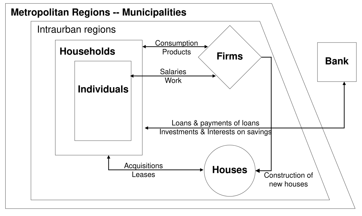
We detailed the model, providing the context of agents and scale and then used the sequence of events to describe the decision-making processes, the related equations, and the supporting literature. Figure 1 depicts the model agents within their spatial hierarchy and the main markets. Each simulation is performed at the level of metropolitan regions. The policy test runs for the metropolitan region of Brasília and its nine surrounding municipalities. Brasília and each municipality is divided by its component intraurban areas – officially census blocks called "weighted areas".6 Houses and firms are located proportionally inside intraurban regions and interact in the markets of labor, goods and services, real estate and credit.
Input data. The data that feeds PS2 comes from official sources and refers basically to the (a) details, location of individuals and households, (b) location of firms, (c) geographic files of municipalities and intraurban regions, (d) state-level data on fertility, mortality, by gender and age, (e) population estimates, human development index, and taxes transferred to municipalities, and (f) general indicators on marriage and car ownership. A full table with sources and descriptive statistics is presented as an Appendix (see Table 4). It is relevant to point out that no data associated with the real estate market enters the model. This means that neither size, quality, nor the prices of dwellings enter the model. All input data is available in the model’s repository.
Agents. PS2 contains individuals who work, commute, age, die and are born, get married, and divorce. Individuals are organized into households (families) and reside in dwellings that have fixed locations. Households may move among residences and are considered as a collective of individuals making decisions on consumption. Firms – also fixed in space – hire individuals, produce and participate in the goods and services market. Construction firms also hire individuals and supply new dwellings in the real estate market. There is a bank that collects deposits, pays interests and offers mortgage loans. Municipalities have actual geographical coordinates, collect taxes on firms and workers, consumption, properties and transactions within their own territory. The model is stock-flow consistent. Workers only receive money from firms. Firms’ revenue comes from sales. Households receive payments from rental and real estate markets paid from other households. The bank makes money from loans and pays interests. Municipalities invest only money collected by taxes.
Scale. PS2 runs monthly from January 2010 to January 2020 in the standard simulation. It may be configured to go up to 2030 and start either in 2000 or 2010. Each simulation is run for a single metropolitan region. We consider the urban core of metropolitan regions, defined and named by the Statistics Bureau as Areas of Concentration of Population (ACPs). The model contains input data for all 46 ACPs of Brazil the model.7 Our study case of Brasília, which is the default run, involves the Federal District (Brasília) and its nine neighboring municipalities.
Sequence of events and details
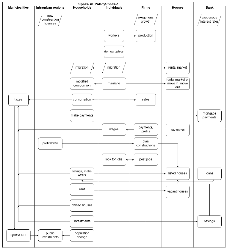
Figure 2 shows a broad sequence of monthly events that are detailed below. Some decision-making involves more than one group of agents. At the beginning of every month exogenous data such as number of new firms and the mortgage interest rate are computed. Workers then engage in production and individual demographics processes occur. Migration is processed following volume of observed exogenous data. However, when entering the model households have to go through the rental market and successfully get a house. Marriage is relevant as it may change internal composition of households and generate endogenous demand for new houses. Next, households consume, firms processes sales and compute consumption taxes. Firms process payments and pay wages. Construction firms calculate most profitable feasible intraurban regions and decide on construction. Then, the labor and real estate markets take place, the latter being mediated by possible mortgage loans. Then, we have the rental market, collection of taxes on real estate transactions, house property, and savings interests paid by the bank to households. Finally, collected taxes are turned into public investments weighted by population change.
- Generator of agents. The model either loads previously saved agents or generates them from official census block data. We also use official intraurban geographically delineated regions. Municipalities are a set of regions. Dwellings are generated so that there is an exogenously assigned number of vacant residences in the model (Nadalin & Igliori 2016). Agents, households and dwellings follow each census block’s population percentage (\(\text{pop}\)) for a given starting year. All houses of the model are allocated to households, thus all houses have owners who are households. The distribution is made so that some households have two houses or more and some have none. Agents are allocated into households and households into dwellings, either as an owner or a rental, randomly distributed.8
- Each region lists the number of available land plots or licenses. Construction firms need to purchase a license in order to build a new property.
- Following exogenous empirical data, new firms enter the simulation.
- Firms produce a homogeneous product using fixed technology (Lengnick 2013). They (\(i\)) update their inventory with goods and services (\(Q_i\)) each month (\(t\)) based on workers (\(l\)) qualification (\(q\)) (Gaffeo et al. 2008) and two exogenous parameters (\(\alpha,\beta\)) (see Equation 1). Construction firms produce dwellings with varying characteristics and location, observing the maximum profitability. However, their production mechanism is the same.
| \[ Q_{i,t} = \sum_{l}^{L} \frac{q_l^{\alpha}}{\beta}\] | \[(1)\] |
- Demographics. Mortality, fertility, new marriages and aging take place according to exogenous probabilistic official data by state. Each agent receives a month of birthdays in which all demographic processes occur. When female agents within fertile age (15-49) give birth, the child is incorporated into the mother’s household. Individuals are relevant in the composition and modification of households and act alone at the labor market. All consumption decisions, however, are made collectively at the household level (see Figure 1).
- Migration and marriage. Migration occurs when necessary to maintain exogenously observed population growth. Households coming into the municipality only stay if they are able to find residence through the real estate market.
Marriage occurs probabilistically. Agents leave their old household (and house property) behind, if not they are the only adult. Otherwise, they bring children (or property) with them, if they have any. Newly formed households persist only if either adult brings a house (or a rental) or if they succeed in the market.
Inheritance. When the last member of a household dies, a search for relatives occur. Members from the household that the deceased originally belonged to receive any wealth or property. When there are no known relatives, any owned property is randomly allocated to another household. - Consumption at the goods and services market. Households choose from an exogenously determined sample size (\(\varsigma\)) either the firm that is the closest or the one with the cheapest product (\(P(.5)\)). The consumption amount is determined by the household’s simplified permanent income (\(PI_{h,t}\)) (Dawid & Delli Gatti 2018), with an extra assumption that expected future income is an average of all previous permanent income (see Equation 2).9 When gathering consumption money, households search first for cash available with each member. If collected cash is not enough to make the permanent income, households try to withdraw from their reserve money (\(R_h\)) or savings (\(S_h\)) from the bank.
The reserve money is simply some cash kept to accommodate fluctuations of wages and balances, which remains in the household’s possession and is not invested in the bank. It provides immediate cash for payment of rentals, loans and consumption. The distinction is only a household internal separation. Reserve money is not invested in the bank, thus receives no interest. It is given as six times the Permanent Income: \(R_h = 6*PI_{h,t}\).
where \(i_t\) is \(r_t/(1+r_t)\) and \(r_t\) is the baseline interest of the economy, \(\overline{Y_{h,t0-t}}\) is the household’s members average monthly income for all available periods and \(w_t\) is the sum of property values, reserve money, savings and loans. Any income the household may have (or gain via rentals or sales) in excess of permanent income is deposited as savings in the bank, except for the reserve money. Simply put, households consume a bit more than total wages if they have savings and a bit less when their total wealth is negative.\[ PI_{h,t} = i_t * \overline{Y_{h,t0-t}} + i_t * \frac{\overline{Y_{h,t0-t}}}{r_t} + w_t * r_t\] \[(2)\]
Note that consumption occurs before firms have paid wages in the current month. Thus, households use resources from last month and their reserve money. In the sequence that follows, wages are paid and monthly housing obligations, that is, rents or mortgage payments, are fulfilled. When the household has no funds from wages, reserve money or savings, it goes with null consumption for that given month. Null consumption is very low for the default configuration of the model. Given the context of Brazil’s current status in 2010s, these numbers are compatible with observed data. At the end of the month, households check whether saving investments are possible. Household savings enable offers on real estate market. - The bank calculates and collects payment for loans. If the household fails to pay in full, the debt accumulates for the next month. Note that the bank pays exogenous baseline economy interest on deposits (\(r_t\)), but applies (also exogenously) market mortgage interest rates on loans.10 We use real observed mortgage rates as default. We also tested nominal and fixed rates at the sensitivity analysis.
- Firms check their revenue, pay taxes and calculate profit. Calculate wages, pay their employees and decide whether to update prices.
Firms’ decision on prices. Blinder (1994) identifies in surveys, a number of different practices firms use when setting prices under uncertainty. His findings support the idea that firms do not evaluate the market every month. PS2 follows Seppecher et al. (2017) in observing the size of the firms’ inventory in order to update prices and does so not every month, but according to an exogenous parameter (\(\zeta\)) (Hamill & Gilbert 2016). If the amount sold in the previous month was above produced quantity, then firms update prices by a markup percentage (\(\pi\)).
Firms’ decision on wages. Firms decide on wages (\(\omega_{l,t}\)) based on total revenue (\(TR_i\)) discounted of taxes on labor (\(tax_l\)) and global unemployment (\(U_t\)) (see Equation 3). In practice, workers’ payments vary according to the firms’ sales and represent their own contributions towards production. The rationale may be considered as a variable bonus attached to firms’ performance.
| \[ \omega_{l,t} = TR_{i,t} * (1 - U_t) * \frac{q^{\alpha}_{l}}{\sum_{l}^{L} q^\alpha} * (1 - tax_l)\] | \[(3)\] |
- Planning new dwellings. Construction firms operate their property planning process considering availability of land plots, profitability, and current supply size. They also check for finished previous construction plans and when listed new properties on the market. First, the firm checks whether their contracted amount of work (\(\sum_h cost\)) is smaller than a fixed number of months (\(n\)) times their current monthly production (\(Q_{i,t}\)). If so, they may start a new construction project. Next, the construction firm checks whether it has enough funds to buy the license plots and separates the regions where it can afford and that actually have available licenses. The firm then tests whether to continue with the construction plans checking probabilistically against global vacancy percentage. This means that the higher the offer on the market the less likely the construction firms start new projects.
In order to evaluate profitability in the regions where there are licenses available, a planned building size and quality are chosen randomly. Next, the firm gets a sampled price of houses that have similar size (within 10 absolute distance) and quality (within 1 absolute distance) for each available region. Cost is calculated as dwelling size (\(H_s\)) times quality (\(H_q\)), times a random productivity factor that is a function of markup (\(f(\pi)\)). Region profitability (\(N_{\pi,m}\)) then is the mean prices of similar dwellings deduced by calculated building cost and license price (\(N_m\)), times lot cost (\(1 + \upsilon\)) (see Equation 4). Given this planning information, the firm evaluates which plan has the most profitability and makes the decision to build at the place and characteristics where it has the highest profit, relative to current mean prices of similar houses. When there are no profitable regions, the firm does not start a new construction.
| \[ N_{\pi,m,t} = \overline{P_{\text{ask},m,t}} - (H_s * H_q * f(\pi) * N_{m,t} * (1 + \upsilon))\] | \[(4)\] |
- Labor market. Neugart & Richiardi (2012) review an initial ABM labor market. A full scale labor market is described by:
They reproduced a number of labor market stylized facts. In PS2 we have opted for a simple labor market (Hamill & Gilbert 2016). All individuals (\(l\)) who are between 16 and 70 years old and out of the job market apply each month. Consumption decisions are all made at the level of the household and the model does not include a pension system, nor unemployment benefits. Brazilian social security rules are complex and vary widely according to employees’ trajectories, sectors, and whether the worker belongs to government or private institutions. Moreover, pension and unemployment benefits cover only formal labor (informal labor accounts for nearly 50% of the population), and are small in value.
Firms (\(i\)) do not enter the market offering positions every month. Rather they probabilistically evaluate whether to do so following an exogenous parameter (\(\iota\)). When in the market, they may either fire a randomly chosen employee, when their profit is negative, or open a position otherwise. Candidates and firms are shuffled. Depending on an exogenous parameter (\(\eta\)), some of the posts available will use a spatial proximity criterion whereas others will make a decision based on qualification of candidates.
Spatial proximity makes sense for Brazilian cities where legislation insists that transport costs should not exceed 6% of wages, with employers bearing any values above this limit. We should also consider that populous Brazilian metropoles are spread across large areas, with low-quality commuting infrastructure, thus making traveling large distances to work costly for both workers and employers.
All positions involve a sample of candidates (\(\sigma\)). The candidates at the pool for each position evaluate the post themselves considering the base wage (\(\Omega\)) paid and the distance from each firm to their residence (\(d_{h-i}\)), mediated by the cost of transport (\(c_{tr}\)). Having access to private transport depends probabilistically on the deciles of income of the candidate’s last wage. That is, higher-income households in Brazil typically owns a vehicle and evaluates time commuting more heavily. As such, those candidates prefer positions that are closer to their residence. Candidates on lower quantiles of income, who have no alternative but public transport also penalizes distance, however, at a lower comparative scale. Although distance and transport are considered as criteria of the labor market, household transportation costs are not included in the model.
Firms’ base wage (\(\Omega\)) is the total amount distributed by the firm on a given month and functions as a proxy that informs the candidate about the size of the firm, which is usually associated with better career paths, salaries and stability. It seems there is no consensus about the firms’ wage decision-making process (Neugart & Richiardi 2012). Additionally, each firm classifies candidates by their qualification (\(q_l\)). All offers are sorted based on the score that considers both candidates and firm parameters (see Equation 5). When firms choose based on proximity exclusively, according to (\(\eta\)), then candidates’ qualification (\(q_l\)) is not considered in the computation of score (\(s_{l,i,t}\)). Firms paying higher wages choose first in descending order. For every pair of firm-candidate – conditional on the candidate having not being chosen earlier – positions are filled successively and firm and candidate leave the market for that month. The market closes when there are no more positions or no more candidates.
\[ s_{l,i,t} = q_l + \Omega_{i,t} - d_{l,h-i,t} * c^{tr}_{l,t}\] - Real estate market. Entering the real estate market is endogenous due to changes in household composition (marriage, divorce) and migration. Households also monthly enter the market exogenously, according to a sample of households (\(\phi\)). However, entering the market does not necessarily means making a new purchase or renting a new house. The offer may not be accepted, the bank may decline the loan, or the new rental may not be better than current dwelling. Houses are listed in the market when vacant.
Prices (\(P_\text{ask}\)) for all properties are updated and those unoccupied are listed and divided between rental and sales market by an exogenous parameter. This means that all unoccupied houses are available in the market. Affordability of both rental and purchasing is the main factor when choosing a house in Brazil. As noted above, more than half of the households would be eligible for federal housing program at the highest level of subsidies.
Rental. In addition to the rental market transactions that might have occurred during migration and marriage procedures, rental market happens first when the main real estate market is run. Households participating in the rental market are sorted by permanent income (\(PI_{h,t}\)). Rentals are initially calculated as a fixed exogenous percentage of the house calculated value. Given a random sample of fixed size (\(\sigma\)), households (\(h\)) choose a rental that is within their budget at price value. When no house that the household can afford is available, the household propose a discounted value on the cheapest rental in the sample. When negotiations are not accepted, households remain at their current house and leave the market. Even when evaluating the market positively, households do not conclude the transaction when their current house is better than the prospective one.
Sales. On the sales market, households are sorted by purchasing power (\(P_{\text{offer}}\)), including an estimate of possible mortgage credit (\(L_h\)). Then, each household tries to buy the best house from their sample (Goldstein 2017), considering size, quality, neighborhood service levels, neighborhood households income, and time on the market. All these elements together compose the price.
Asking prices. The asking price is calculated considering the dwelling size, quality (\(H_{s,q}\)), and the neighborhood quality of life index (\(N\)) which differs by region (\(m\)) and changes monthly depending on taxes invested and population proportion (see below item 15)(Rosenthal & Ross 2015). This follows the hedonic price literature that breaks down house value as the cumulative sum of its characteristics (Malpezzi 2002; Rosen 1974). Additionally, an extra comparative effect of neighborhood – also shown in the sensitivity analysis – is added to the default configuration. A parameter (\(\tau\)) brings the influence of a normalized index of neighborhood households average income (\(N_q\in[0,1]\)) into prices (Ge 2017). Finally, a discount for time on the market is incorporated into prices with a bounded value (\(\gamma\)) and a decay factor (\(\kappa\)), depending on the number of months the property has been listed (\(T\)) (see Equation 6).
Bank mortgage criteria. The bank follows three simple criteria to provide mortgage loans: (a) the bank needs to have a positive balance; (b) the household cannot have a current mortgage, and (c) total loans already offered cannot be higher than the percentage of total deposits (\(\nu\)) as established by monetary authorities. When those criteria are valid, the amount (\(L_h\)) the bank provides depends on the maximum capacity of monthly payment the household can make, restricted by a limit (\(\chi\)) of permanent income (\(PI_h * \chi\)) times the maximum number of months (\(m\)) (360) or the number of months before the oldest member of the family reaches 75 years old, so that \(L_h = PI_h * \chi * m\)
Negotiation. When the property’s price is below the household’s savings, the transaction is made with final price (\(P\)) set as a simple average of asked price and household’s savings (Dweck et al. 2020). When a property’s price requires a mortgage loan (\(L_h\)), the buyer requests the loan on the difference between savings and asked price. If successful in getting the mortgage loan, the offer price (\(P_{\text{offer}}\)) is savings plus estimated mortgage (see Equations 7 and 8). Otherwise, when the loan is declined by the bank, the household leaves the market. When the savings are below the asked price, but above an exogenous parameter limit (\(\rho_{-}\)), the buyer makes an offer with their total savings. The chance that the seller will accept depends probabilistically on the size of the supply market (see Equation 6). When both savings and savings with mortgage are below property asked price, and the discount is not possible or accepted, households try the next house on the list.
Constraints. There are certain constraints imposed on prices. The ratio savings, price is upper-bounded by an exogenous parameter (\(\rho_{+}\)) and there is a loan-to-value parameter (\(\text{LTV}\)) on mortgage requests (see Equations 9 and 10).
Rental and mortgage payments Whenever the household does not have enough resources to pay for rent, tenants default on rent and landlords bear the loss. These defaults on rent are very low on a typical simulation run and are compatible with empirical data. When households default on mortgages, the bank incorporates the temporary loss and tries to recover it in posterior months.
| \[\begin{gathered} P_{\text{ask}} = H_{s,q} * N_{m,t} * (1 + \tau * N_q) * ((1 - \gamma) * e^{\kappa * T} + \gamma) \end{gathered} \] | \[(6)\] |
| \[ P_{\text{offer}} = S_h \lor S_h + L_h \text{ if } P_{\text{ask}} < P_{\text{offer}} \] | \[(7)\] |
| \[ P = ( P_{\text{ask}} + P_{\text{offer}}) /2 \] | \[(8)\] |
| \[L_h / P <= \text{LTV} \] | \[(9)\] |
| \[ \text{if } P_{\text{ask}} / P_{\text{offer}} > \rho_{+} \longrightarrow P = P_{\text{offer}} * \rho_{+} / 2 \] | \[(10)\] |
| \[ \text{if } P_{\text{ask}} > S_h > \rho_{-} \longrightarrow P = S_h | P(\sum \text{Listed} / \sum h) \] | \[(11)\] |
- Decision on moving. Jordan et al. (2012) list seven reasons why households change residences. Those include changes in socioeconomic status (such as losing jobs), and searching for better quality of life in a better neighborhood. As a decision made by the household unit, the financial power of its members influences the capacity to acquire larger and better houses. Households will move to the best dwelling (Goldstein 2017)) when at least one member is employed. In the rare case that all adult members are unemployed, households will move to the worst house they own and sell the best one in order to capitalize and adjust their familial budget. Moving occurs endogenously within PS2 when a household status change, due to marriage, for example, or a migration event. Exogenously, the household will at times participate in the real estate market, but the purchasing and moving only happens when the full process occurs successfully.
- Households invest. The bank keeps the date to calculate interest at the exogenous rate (\(i_t\)).
- Municipalities invest in Quality of Life Index improvement (\(N_{m,t}\)). All taxes collected: consumption, labor, firm profits, house transactions and house taxes, are transferred to the municipalities budget according to tax rules distributions in Brazil, following the original model (Furtado 2018). Investments are linear and transformed via an exogenous municipal efficiency index (\(\psi\)) and population (\(\text{pop}_m\)) difference, so that: \(N_{m,t} += \sum_{m} tax_t * \psi * \text{pop}_{m,t-1}/\text{pop}_{m,t}\). The index is thought of as a proxy for the Municipal Human Development Index (M-HDI) and it represents the municipal capacity to collect taxes – given by the dynamics of markets within its boundaries – weighted by the proportion of its population. Hence, areas that have markets that are proportionally more dynamic invest more in infrastructure and amenities. All municipalities start with their observed M-HDI in 2010. \(\psi\) is calibrated so that values maintain a resemblance with M-HDI. Municipal investments (or lack thereof) impact house prices as they reflect these changes in urban quality. Implicitly, households living in places with higher QLI enjoy a better level of services and amenities.
- Statistics and output are calculated and saved. The Gini coefficient is based on households’ permanent income (see Equation 2). That means that average household income as well as housing property or mortgages enter the calculation. GDP is calculated as the sum of firms’ revenues by municipality and aggregated for the metropolitan region.
Policy experimental design
The policy experiment is applied using endogenously collected taxes by municipality (\(m\)). Instead of investing full budget to an improvement in quality of life (\(\sum_{m} tax\)), a percentage (\(\delta\)) is diverted to either one of three policy experiments (Table 1). This endogenous mechanism guarantees a high degree of comparability among the three tested policies.
When applying a policy, the first action is to register all households whose permanent income (\(PI_{h,t}\)) has been below an exogenous quantile (\(\theta\)) of the households of the metropolitan region in the previous year and currently resides within the municipality. Households are then sorted according to permanent income so that the poorest of all municipal households is the first in line (see Table 1).
- Property acquisition and distribution. The municipality lists all properties in the region that construction firms have finished but have not sold yet and sorts them by the cheapest to the most expensive. The list of households registered includes only those who do not own any property. Then, the municipality purchases the property from the selling firm, and transfers the property to the household next on the list. The municipality buys and transfers houses for as long as the monthly available allotted funding, properties, and households last. Benefited households do not pay for the houses they receive.
- Rental payment vouchers. The municipality lists all households that do not own any properties and are in the policy register. Thus, as long as there is enough funding and households the municipality issues 24-month rental vouchers that should cover the current household rental price. Rental vouchers are attached to the current rental contract. If the household decides to leave the residence, it gives the remaining vouchers, if any, back to the municipality. Households can only apply for new vouchers after they have expended all previously received and the criteria to be listed still hold.
- Monetary aid. In this policy scenario, the municipality divides all monthly available funding equally into a single payment for all households listed at that moment in the policy register. Households are free to use the funds received.
- No-policy – baseline. In this case, no money is invested in policy and all resources go into investment in municipal quality of life (\(N_m\)).
| Policies | \(\delta\) portion of municipal budget \(\sum_{m} tax\) | Benefit period | Amount received |
|---|---|---|---|
| Property acquisition | .2 | Permanent | The house itself |
| Rental payment vouchers | .2 | 24 months | Rental value |
| Monetary aid | .2 | Current month | Variable |
| No-policy baseline | 0 | ||
Verification, Calibration and Sensitivity Nnalysis, and Validation
Computational analyses are always subject to possible errors of execution or actions that differ from the original intention of the modeler (Galán et al. 2009). In order to avoid the occurrence of such errors, programmers need to verify that the code executes as intended. Some procedures applied to PS2 aimed at warranting processes ran as expected.
We observed 66 different outputs of the model to precisely follow results and changes from changing parameters, procedures or code. Moreover, we included a series of assert commands throughout the code – available at a public repository – to make sure of the variable values at key points. Finally, we ran specific tests to check, for example, whether construction firms actually build new houses, banks effectively loan to families or whether there is any household without a current address. Specifically, we tested the flow of financial resources among agents to ensure that the model was cash-flow consistent.
We aimed to validate PolicySpace2 through a series of successive steps. First a series of macroeconomics indicators have to behave reasonably within expected values. Even though these indicators have been calibrated, they happen to be within reasonable boundaries simultaneously. This means that the Gini coefficient, inflation, and unemployment among other indicators are all sensible.
Brasília – which is our baseline case – had a Gini coefficient of 0.4705, total inflation for the 10-year period is 43.32%, and unemployment 12.39% which are within the expected values of Brazil. Apart from that, extensive variations in the parameters (or the metropolitan regions) resulted in different values but did not lead to the collapse or exponential behavior of the results of the model.
Most rules, procedures, and parameters come from literature or data. Firms’ decisions on prices, wages, and production, for example, are based on previous works. Price setting in the real estate market follows hedonic and urban economics baselines with also some support from urban studies. The labor market does not have a clear predecessor, despite the contributions of Neugart & Richiardi (2012), but it is based on commuting costs and activities’ time allocation. Parameters follow observed data as much as possible.
Moreover, certain new rules implemented in PolicySpace2 are tested in the sense that they can easily be turned on and off. Specifically, we tested three structural rules and investigated eight different aspects of the model in order to comprehend the underlying mechanisms better. We also performed sensitivity analysis on model parameters.
- Proximity to labor market (\(\eta\)). We tested the influence of \(\eta\) from 0 to 1. When \(\eta==0\) distance is not considered in the labor market and all candidates are selected exclusively based on their qualification. When \(\eta=1\), candidates are selected based on distance only. The analysis suggests that most values between the extremes are reasonable in the sense that unemployment and the other indicators remain stable. When \(\eta\) is set in the extremes of 0 or 1, unemployment is much larger, GPD is lower, and total household commuting is much lower.
- Neighborhood effect on house prices (\(\tau\)). We tested \(\tau\) in the interval 0 to 5. When \(\tau=0\) the rule is not in effect and the neighborhood average income – a proxy for neighborhood value and perception – is not included in price calculation. As a result, prices are lower and GDP is higher. Perception of neighborhood value for real estate prices, however, is relevant for price composition (De Nadai & Lepri 2018), thus our default value \(\tau=3\) includes a moderate influence of the neighborhood in prices.
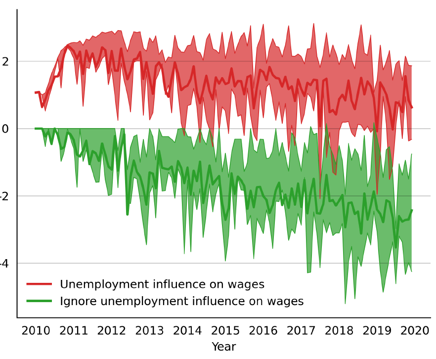
- Global unemployment (\(U_t\)) as a factor on firms’ wage setting. We tested the presence of unemployment on firms’ mechanism of wage-setting. Mostly the presence of the rule influences the finances of the firm providing it with additional money availability that enables the firms to counteract high volatility of demand (see Figure 3).
After verifying the code and calibrating the parameters, a thorough sensitivity analysis was applied to the final model. A sensitivity analysis aimed to understand the mechanisms behind the model and interactions across different markets and agents. In total, we ran 5,573 simulations with more than 244 unique configurations of parameters. All parameters were tested with a variation of combinations. This helped verify the robustness of results as well as to gain insights into the operational emergence of model results.11 Specifically, we tested all five taxes with different values for the parameters. The results showed levels of magnitude for the results, without however changing the typical trend of indicators.
Regarding the purpose of the model – to investigate "alternative household poverty alleviating mechanisms", we tested the policy experiment in four other metropolitan regions. All tested rules and parameters maintained the bulk of the results presented with similar observed trends (see Table 3).
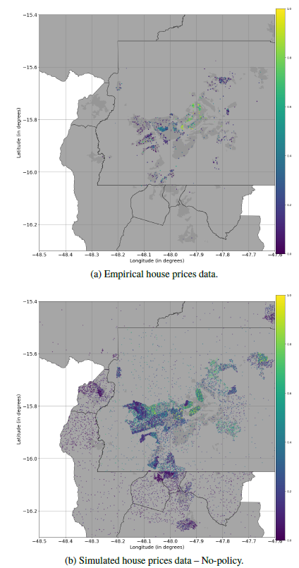
Validation itself was done by comparing data collected for the Brasília real estate market that never went into the model. It was gathered independently from listing offers available on internet sites mostly during 2020. The empirical data contains 23,103 observations across 61 neighborhoods with a median house selling for R$ 750,000 with three bedrooms in 126 square meter and R$ 6,011 per square meter. The model data however, only uses information from Census and official data, mostly from 2010 (although it is also possible to run with 2000s data).
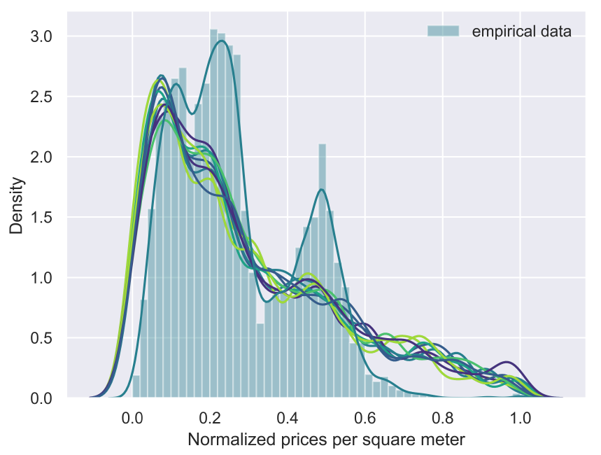
We compared normalized prices over space for Brasília using data from the last month of the simulation (see Figure 4). The comparison aimed to provide evidence that generated relative prices mechanisms across the metropolitan region were compatible with the observed data. Results were spatially similar in the sense that the simulation was able to replicate a more expensive area in the central, planned area of Brasília, and lower priced areas in the neighboring municipalities and in the Western portion of Brasília. Second-tier cluster of prices, especially in the northeastern area were more expensive in the simulation compared with empirical data. This led to a more homogeneous distribution in simulated data compared to a more clustered, double-peaked distribution for the empirical data (see Figure 5). Observed prices were more volatile and ragged comparatively to simulated prices which were more continuous with less pronounced peaks. Simulated data also followed the location of firms.
However, considering that the description of properties size, quality or price is not included in the model, the similarity we were able to achieve, given a market that includes heterogeneous properties (central, small one-bedroom high valued properties, but also, large, distant, sophisticated properties) seem to be sufficient to hold the comparison and thus serve the purpose of the model.
Finally, the general centralized, richer configuration of the metropolitan region with higher unemployment, lower wages, and poorly more homogeneous peripheries is also reproduced in the simulation (see Table 5).
Results
Results clearly show that from an endogenous perspective, the best policy seems to be Monetary aid, e.g., the distribution of a lower amount of aid directly to a larger number of households (see Figure 6).
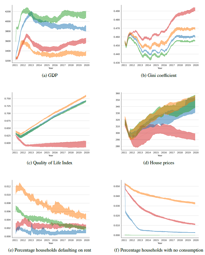
Given the endogenous amount of funding distributed towards the policies, it is up to the internal processes of the model how to push the economy forward. When the Monetary aid policy is introduced, more households are able to consume larger quantities from the goods and services market. The resulting sales and revenues allow for firms to pay higher wages. This leads to an expected slight increase in prices. Even then, a smaller number of households fail to pay their rents or mortgages or go a month without consuming goods and services. Overall, this leads to much lower inequality with higher GDP achievement.
The Rental voucher policy is a somewhat intermediate alternative with a much smaller number of households being supported. On average, Monetary aid policy helps 2,358.05 households monthly per municipality, compared to 47.5 for Rental vouchers and 12.37 for the Property acquisition program.12 Even then, Rental policy seems to achieve lower inequality which is comparable to that of the Monetary aid, although with not as much an increase in GDP.
Property acquisition seems to be the policy that performs worst. It lowers overall mean household permanent income compared to the other policies and to the No-policy baseline. Further, it sharply increases inequality – as it provides an asset to a small number of households. On the positive side, it seems to increase firms (construction firms) total assets in a more pronounced way than the other two policy alternatives as well as helping to decrease house prices.
The No-policy baseline results are provided as a comparison of the performance of the model. Consider that whereas the funding separated for the policy programs is reinvested in absolute terms, the investment when there is No-policy is made in full via the linear transformation of the \(\psi\) parameter. Conversely, among the policies’ alternatives, the exact same processes, procedures, and parameters run each policy scenario. This makes the policy alternatives highly comparable.
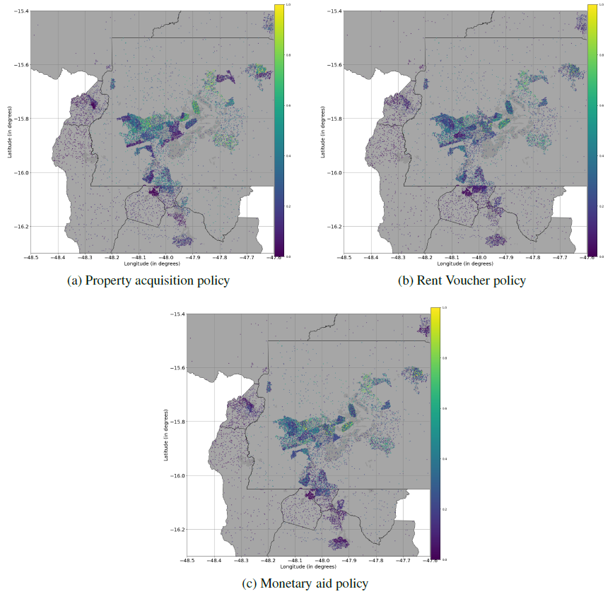
Considering a spatial analysis of house prices over the policy alternatives (see Figure 7), Property acquisition and Monetary aid seem to cause a slightly more dispersed and homogeneous distribution of prices, compared to Rent voucher and No-policy baseline, especially when the Western populous region of Brasília and its southern border are considered. These results are confirmed by the analysis of the Gini coefficient for each municipality for the baseline case versus the application of the policy experiments (see Table 2).
| Municipalities – Brasília RM | Property | Monetary | No-policy | Rental |
|---|---|---|---|---|
| Águas Lindas de Goiás | 0.4138 | 0.3538 | 0.3753 | 0.3628 |
| Cidade Ocidental | 0.4238 | 0.3863 | 0.3961 | 0.3888 |
| Formosa | 0.4317 | 0.3850 | 0.3996 | 0.3911 |
| Luziânia | 0.4484 | 0.3961 | 0.4069 | 0.4002 |
| Novo Gama | 0.4427 | 0.3761 | 0.3994 | 0.3826 |
| Padre Bernardo | 0.3905 | 0.3414 | 0.3694 | 0.3559 |
| Planaltina | 0.4451 | 0.4105 | 0.4303 | 0.4235 |
| Santo Antônio do Descoberto | 0.3953 | 0.3436 | 0.3597 | 0.3430 |
| Valparaíso de Goiás | 0.4444 | 0.3983 | 0.4179 | 0.4051 |
| Brasília | 0.4854 | 0.4467 | 0.4619 | 0.4521 |
Policy scenarios were also run for longer periods 2010–2030, maintaining certain exogenous data such as mortgage rates constant. Additionally, a very long run, based on census 2000 data was run for the period 2000-2030, using the same parameters that were calibrated for the 2010–2020 default configuration. In both cases, the Gini coefficient maintained a trajectory of increasing inequality for implementation of the Property acquisition policy whereas it did not affact the other alternatives. GDP, however, also incrased for Property acquisition, whereas a declining path was observed in the other scenarios.
The robustness of the results were confirmed when we tested the policy alternatives for four other middle-sized metropolitan regions of Brazil, from different regions, and with unique spatial, household, and qualification characteristics. Averaging results of six indicators for the full period and 20 simulation runs for each policy test are presented in Table 3. The Gini coefficient was lower on average for Monetary aid policy compared to No-policy scenario for all cities, at the same time that GDP was higher. Household consumption was also higher for all cities. All policies generated higher inflation over the 10-year period, except for Porto Alegre. Unemployment did not seem to be affected by policy, with results remaining stable for all cities across all policies. Finally, house prices seemed to be lower for policy implementations, with more pronounced results in the case of Property acquisition, except for Porto Alegre that observed the lowest price on average for the Rent voucher case.
| Gini Coefficient | ||||
|---|---|---|---|---|
| Property | Rent voucher | Monetary aid | No-policy | |
| Brasília | 0.47 | 0.45 | 0.45 | 0.46 |
| Belo Horizonte | 0.42 | 0.41 | 0.4 | 0.41 |
| Campinas | 0.44 | 0.42 | 0.41 | 0.42 |
| Fortaleza | 0.44 | 0.42 | 0.42 | 0.43 |
| Porto Alegre | 0.44 | 0.43 | 0.42 | 0.43 |
| GDP | ||||
| Property | Rent voucher | Monetary aid | No-policy | |
| Brasília | 3410.3 | 3768.7 | 3814.3 | 3298.3 |
| Belo Horizonte | 5664.1 | 6174.4 | 6326.6 | 5520.1 |
| Campinas | 3545.7 | 3782.7 | 3905.1 | 3312.4 |
| Fortaleza | 3684.9 | 3954.9 | 4025.4 | 3545.3 |
| Porto Alegre | 4052.6 | 4258.0 | 4341.3 | 3882.2 |
| Household consumption | ||||
| Property | Rent voucher | Monetary aid | No-policy | |
| Brasília | 0.25 | 0.31 | 0.31 | 0.25 |
| Belo Horizonte | 0.28 | 0.34 | 0.35 | 0.28 |
| Campinas | 0.32 | 0.38 | 0.4 | 0.31 |
| Fortaleza | 0.29 | 0.34 | 0.35 | 0.29 |
| Porto Alegre | 0.31 | 0.36 | 0.37 | 0.31 |
| Price index | ||||
| Property | Rent voucher | Monetary aid | No-policy | |
| Brasília | 1.39 | 1.49 | 1.48 | 1.38 |
| Belo Horizonte | 1.74 | 1.96 | 2.01 | 1.71 |
| Campinas | 1.56 | 1.76 | 1.83 | 1.55 |
| Fortaleza | 1.41 | 1.54 | 1.57 | 1.39 |
| Porto Alegre | 1.57 | 1.81 | 1.87 | 1.58 |
| Unemployment | ||||
| Property | Rent voucher | Monetary aid | No-policy | |
| Brasília | 0.11 | 0.11 | 0.11 | 0.11 |
| Belo Horizonte | 0.13 | 0.13 | 0.13 | 0.13 |
| Campinas | 0.06 | 0.06 | 0.06 | 0.06 |
| Fortaleza | 0.1 | 0.1 | 0.1 | 0.1 |
| Porto Alegre | 0.08 | 0.08 | 0.08 | 0.08 |
| House prices | ||||
| Property | Rent voucher | Monetary aid | No-policy | |
| Brasília | 308.56 | 322.86 | 320.71 | 327.56 |
| Belo Horizonte | 223.44 | 225.13 | 222.86 | 225.78 |
| Campinas | 255.45 | 254.76 | 249.55 | 260.09 |
| Fortaleza | 256.47 | 267.39 | 266.32 | 270.93 |
| Porto Alegre | 261.24 | 261.14 | 262.09 | 266.59 |
Intuition, discussion and future work
One of the essential differences among the policies tested is that Monetary aid is provided for a larger number of households relative to Property acquisition and Rental voucher. Rental voucher performed close to Monetary aid and further from Property acquisition for different indicators. In practice, this would mean that a social welfare policy program, such as the Bolsa Família, instated in 2003, and expanded in subsequent administrations, may be more beneficial than the housing program MCMV. Specifically to provide affordable housing, rental mechanisms may be a better policy compared to property distributions.
We believe that a mechanism that plays a relevant role in the simulation is that when buying houses and handing them over to households immobilizes capital whilst supporting construction firms. This capital then returns back to the system as savings (which may be spent on goods), increases the housing stock and construction workers’ salaries. However, feedback might be slower than Monetary aid and Rental voucher policies.
Furthermore, this capital immobilization impacts tax collection. The dynamics of Monetary aid and Rental vouchers enable tax collection trends to be maintained. Property acquisition, however, does not seem to maintain the level investments on municipalities, thus affecting the Quality of Life Index. This, in turn, also affects house prices.
The analysis of alternative policy scenarios is made considering the perspective of municipalities and local policy-makers. The question often posed by politicians is: "given a set of financial resources, which policy will mostly benefit citizens?" Along with this question, we believe that PS2 contributes with the ability to observe endogenous effects across different aspects of social life. As such, policies across different areas (housing or social benefits) may be evaluated relative to one another.
Providing housing alone may not be sufficient if the benefit does not include jobs and services and access to the city, as shown by the policy program implemented through 2009–2019. Moreover, houses’ characteristics make it an expensive good (Arnott 1987) in a thin, volatile (Glaeser & Nathanson 2017), complex market.
All things considered, if the municipality is seeking a specific housing policy, these simulations suggest that a Rental voucher may be more beneficial. This both provides families with house security and grants households mobility (De Nadai & Lepri 2018), whilst keeping municipal investments relatively low. However, if the municipality is not seeking a housing policy per se, but a general policy to invest its financial resources, a Monetary aid alternative might be better.
PS2 is already a complex model. Nevertheless, we are considering a number of future developments. Firstly, the model can always be improved, and interactions more detailed. For PS2 specifically, this might involve the credit market, firms, and transportation and education systems. Secondly, we also intend to publish further material that would include results for all 46 metropolitan regions, along with policy comparisons for all of them. Such publication would also include more details of the comprehensive sensitivity analysis we have performed. Finally, in terms of policy analysis, we would like to test whether simultaneous policies at different amounts of percentage of the available budget would make an optimal decision mix. Policies could also be financed exogenously, for example, by the Federal government.
Final Considerations
We applied an empirical, economic, spatial, open-source agent-based model that uses official data to generate households, firms, and municipalities that interact in the markets of labor, credit, real estate and goods, and services to endogenously test alternative, cross-sectors policy programs. Poor households – those from the lowest fifth of the distribution – are registered at their municipalities and organized according to their observed income levels. Municipalities collect funds via taxes on consumption, labor, firm’s profits, investments, property transactions, and tax on properties. Regularly municipalities invest in a general improvement of quality of life. When applying policies, the municipal body alternately reserves a fifth of its funds to (a) acquire and distribute properties for poorest households, (b) provide 24-month rental vouchers or (c) simply divide the monthly available resources with all of the registered households. Results hold for a number of different parameter intervals, rules and applied processes, and metropolitan regions tested. Within the context of the model, the monetary aid performs better than the alternatives in nearly all of the indicators used. Mainly, monetary aid reduced inequality at the same time that it increased overall economic output.
PS2 benefits from previous modeling work on macroeconomics, housing markets, transport, and land-use change. We tried to incorporate most of the benchmarks and procedures both in modeling and in communicating. The confidence in PS2 comes from the sustainable robustness it has shown on top of added mechanisms, data, parameters, and markets. Confidence in the results come from the theoretical comparison between the alternative choices.
The aim of the paper is not, however, to recommend an extinction of housing acquisition and distribution to poorest families. We believe PS2 only demonstrates that a given policy – however focused it might be – might endogenously contribute more to the economy when dispersing more funds, rather than concentrating them in fewer households.
Nevertheless, when facing a specific housing program with strict lack of shelter, rental vouchers might benefit a larger number of people and result in greater gains for the society as a whole.13
Finally, we believe that the contributions of PS2 surpasses the policy analysis itself. We have provided a comprehensive empirical, documented, and robust agent-based model that is open source and modular and can facilitate further research. The difficulties in working with PS2 and other ABMs is probably due to its flexibility and adaptation. We believe PS2 is nearly ready to be expanded and used in a series of other analyses, for instance: (a) urban mobility – given location of workers and firms, along with endogenous characteristics of both; (b) social mobility – given the dependence of workers productivity on qualification and its current static nature; (c) migration and newly formed households; (d) inheritance – for analyses with longer periods of time; (e) a more detailed credit mechanism and authority ruling; (f) urban zoning and regulation; (g) amenities, neighborhood perceptions and its influences on prices. Given proper data and initial agent generation, PS2 might also serve the purpose of fostering understanding of long-term market prices and behaviors.
Model Documentation
- PS2 runs in
python v.3.8.5and requires spatial libraries, such asshapely, gdal, descartes, fiona, and geopandas=0.7.0, and numerical and fast-processing ones, such asnumba, joblib and scipy. - Fork and clone the repository from ComSES Open ABM https://www.comses.net/codebase-release/bc5b116a-5fdf-4b6f-837a-a7978ab34268/.
- After installation of requirements, make sure to alter
conf/run.pyand adjustOUTPUT_PATHfor your saving folder. - You may use
–runsand–cpusto specify number of runs and CPUs to be used in a simulation. Default uses all cores in your computer. - A simple run with two CPUs and for 10 simulation runs is run with the command:
python main.py -c 2 -n 10 run - Sensitivity analysis on parameters may be run with
python main.py sensitivity ALPHA:0:1:7, for example. It may also include options -c and -n. The syntax is
sensitivity PARAM:INITIAL_VALUE:LAST_VALUE:NUMBER_INTERVALS - To test for the Policies, you may run:
python main.py sensitivity POLICIES - Plots are generated automatically. Some options for running, saving and plotting are available in the
conf/runfolder.
Notes
- Morandi (2016) estimates construction represented 1.8 of Brazilian GDP in 2014, and a total net fixed capital stock of nearly 8,000,000 (Million R$ of 2010).↩︎
- PolicySpace2 full code is available at GitHub: Github.com/BAFurtado/PolicySpace2↩︎
- Banco Nacional de Habitação – BNH, in Portuguese↩︎
- Minha Casa Minha Vida – MCMV, in Portuguese.↩︎
- Motorization rate is at 37.3%↩︎
- Weighted areas are referred to as "Áreas de Ponderação" in Portuguese by the the Brazilian Statistics Bureau (IBGE).↩︎
- Please, check the repository for a full list.↩︎
- Parameters and their standard value are described in the Appendix.↩︎
- Permanent income is "a linear function of current and expected future incomes and of financial wealth." (Dawid & Delli Gatti 2018, p. 78)↩︎
- See Ge (2017) for an example of an endogenous mortgage rate mechanism.↩︎
- Please note that PS2 comes with a ‘sensitivity’ run that automatically tests Boolean, quantitative parameters, tax rules distribution, a run with all metropolitan regions, and all policies. The code encloses built-in runs that provide output as comparative plots.↩︎
- That considers the standard run parameter of 1% of the population of the metropolitan region and the policy coefficient (\(\delta\)) of .2 over the available funding for each municipality to apply on the policy. Alternative values for \(\delta\) did not alter the results.↩︎
- We also noticed that poor families recurrently – although slightly diminishing in numbers – accessed the Rental program. As such, other structural policies might be needed.↩︎
Appendix
Input data
See Table 4 for the parameter values used on the standard simulation run.
| Input Data for Metropolitan Region of Brasília | Source | Period | Observations * cols | Max | Min | Mean | Standard-deviation | Observations |
|---|---|---|---|---|---|---|---|---|
| Urban proportion | IBGE sidra:table 202 | 2010 | 10 | 1 | 0.3898 | 0.8824 | 0.1848 | Brasília + 9 mun. |
| Females per mun. per age | IBGE sidra: table 1378 | 2010 | 10 (mun.) * 101 (year of age) | 30467 | 0 | 1772.6 | 2964.39 | Ages from 0 to 100. Statistics for all ages. |
| Males per mun. per age | IBGE sidra: table 1378 | 2010 | 10 (mun.) * 101 (year of age) | 27115 | 0 | 1653.78 | 2846.47 | Age from 0 to 100. Statistics for all ages. |
| People per region per gender per age | IBGE: census blocks | 2010 | 17978 | 1367 | 0 | 192.47 | 194.08 | |
| Number of members per family per region | IBGE: census blocks | 2010 | 89 | 3.89 | 2.42 | 3.41 | 0.26 | |
| Population estimates | IBGE | 2001-2019 | 10 * 17 | 3039444 | 22108 | 353497.94 | 99428.83 | Statistics for all years. |
| Geographic shapefiles | IBGE: geoftp | 2010 | 89 | Intraurban regions. Brasília: 51, neighboring mun: 38 | ||||
| Number firms per region | Ministry of Labor: RAIS | 2012 | 89 | 7446 | 3 | 660.84 | 1106.12 | |
| Number firms per region | Ministry of Labor: RAIS | 2017 | 89 | 8299 | 3 | 750.27 | 1158.48 | |
| Cumulative prob. highest level instruction per region | IBGE: census blocks | 2010 | 89 | 1 | 0.1814 | 0.8177 | 0.0771 | 5 qualification levels |
| Mortgage real interest | BACEN: series 25497 | 2010-2020 | 241 | 0.016 | 0.0001 | 0.0076 | 0.0034 | |
| Fertility per age per calendar year | IBGE | 2010-2020 | 35 (age years) * 21 (calendar years) * 2 states | 0.0306 | 0.00015 | 0.0099 | 0.00125 | State-level data age 15-49 |
| Mortality per gender per age per calendar year per state | IBGE | 2010-2020 | 2 (gender) * 111 (age years) * 21 (calendar years) * 2 states | 1 | 0.000105 | 0.1011 | 0.02406 | State-level data age 0-110 |
| FPM: municipal tax transfers | Ministry of Economics | 2000-2016 | 171 | 135441938.2 | 2206964.75 | 22061509.85 | 22369980.67 | |
| HDI-M | FJP and Ipea | 2010 | 10 | 0.824 | 0.651 | 0.7087 | 0.0516 | atlasbrasil.org.br/2013/ |
Parameters
See Table 5 for the parameter values used on the standard simulation run.
| Parameters | Code name | Standard values | Tested intervals |
|---|---|---|---|
| \(\text{pop}\) | percentage of population | .01 | [.005, .03] |
| \(\alpha\) | productivity exponent | .6 | [0, 1] |
| \(\beta\) | productivity magnitude divisor | 10 | [1, 36] |
| \(\iota\) | labor market | .75 | [0, 1] |
| \(\eta\) | percentage distance hiring | .3 | [0, 1] |
| \(\phi\) | perc. entering real estate market | .0045 | [0, .05] |
| \(\sigma\) | hiring sample size | 20 | [1, 100] |
| \(\varsigma\) | size market | 5 | [1, 20] |
| \(\rho_{+}\) | capped top value | 1.3 | [1, 1.5] |
| \(\rho_{-}\) | capped low value | .7 | [.5, 1] |
| \(\tau\) | neighborhood effect | 3 | [0, 5] |
| \(\gamma\) | max offer discount – lower bound | .6 | [.5, 1] |
| \(\kappa\) | on market decay factor | -.01 | [0, -.05] |
| \(\pi\) | markup | .15 | [0, .3] |
| \(\psi\) | municipal efficiency index | .00007 | [.00001, .0001] |
| \(\nu\) | max loan bank percentage | .7 | [0, 1] |
| \(\chi\) | loan payment to permanent income | .5 | [0, 1] |
| \(n\) | construction cash flow – n. months | 24 | [1, 36] |
| \(\upsilon\) | lot cost | .15 | [.01, .3] |
| \(\zeta\) | sticky prices | .7 | [.1, .9] |
| \(\delta\) | policy coefficient | .2 | [0, .3] |
| \(\theta\) | policy quantile | .2 | [.1, .3] |
References
ALONSO, W. (1964). Location and Land Use: Toward a General Theory of Land Rent. Cambridge, MA: Harvard University Press.
ANDERSEN, H. S. (2011). Motives for tenure choice during the life cycle: The importance of non-Economic factors and other housing preferences. Housing, Theory and Society, 28(2), 183–207.
ARENTZE, T. A., Ettema, D., & Timmermans, H. J. P. (2010). Incorporating time and income constraints in dynamic agent-based models of activity generation and time use: Approach and illustration. Transportation Research Part C: Emerging Technologies, 18(1), 71–83.
ARNOTT, R. (1987). Economic theory and housing. Handbook of Regional and Urban Economics, 2, 959–988.
ARTHUR, W. B. (1994). Inductive reasoning and bounded rationality. The American Economic Review, 84(2), 406–411.
AXTELL, R. (2013). Endogenous firms and their dynamics. Tech. rep., Working paper, http://www.acefinmod.com/docs/esrc/axtell-firms.pdf.
AXTELL, R., Farmer, D., Geanakoplos, J., Howitt, P., Carrella, E., Conlee, B., Goldstein, J., Hendrey, M., Kalikman, P., & Masad, D. (2014). An agent-Based model of the housing market bubble in Metropolitan Washington, DC. Available at: https://apo.org.au/sites/default/files/resource-files/2014-05/apo-nid172196.pdf.
BAPTISTA, R., Farmer, J. D., Hinterschweiger, M., Low, K., Tang, D., & Uluc, A. (2016). Macroprudential policy in an agent-based model of the UK housing market. Working Paper No. 619, The Bank of England. Available at: https://www.bankofengland.co.uk/working-paper/2016/macroprudential-policy-in-an-agent-based-model-of-the-uk-housing-market.
BETTENCOURT, L. M. A. (2013). The origins of scaling in cities. Science, 340(6139), 1438–1441.
BLINDER, A. S. (1994). 'On sticky prices: Academic theories meet the real world.' In N. G. Mankiw (Ed.), Monetary Policy (pp. 117–154). Chicago, IL: The Univerisity of Chicago Press.
BOURASSA, S. C., Cantoni, E., & Hoesli, M. (2007). Spatial dependence, housing submarkets and house price prediction. Journal of Real Estate Finance and Economics, 35, 143–160.
BOURASSA, S. C., Hamelink, F., Hoesli, M., & MacGregor, B. D. (1999). Defining housing submarkets. Journal of Housing Economics, 8(2), 160–183.
BRUECKNER, J. (1987). 'The structure of urban equilibria: A unified treatment of the Muth-Mills model.' In E. Mills (Ed.), Handbook of Regional and Urban Economics (Vol. 2, pp. 821–845). Amsterdam, NL: Elsevier.
BRUECKNER, J. K., Thisse, J. F., & Zenou, Y. (1999). Why is central Paris rich and downtown Detroit poor? An amenity-based theory. European Economic Review, 43(1), 91–107.
CARSTENSEN, C. L. (2015). An agent-based model of the housing market. Master Thesis, University of Copenhagen, Copenhagen, Denmark. Available at: https://www.bvc.dk/media/1194/an-agent-based-model-ofthe-housing-market-thesis.pdf.
CAUSA, O., Woloszko, N., & Leite, D. (2019). Housing, wealth accumulation and wealth distribution: Evidence and stylized facts. OECD. Available at: https://www.oecd-ilibrary.org/economics/housing-wealth-accumulation-and-wealth-distribution-evidence-and-stylized-facts_86954c10-en.
DAVIES, A. (2013). “Right to buy”: The development of a conservative housing policy, 1945–1980. Contemporary British History, 27(4), 421–444.
DAVIS, M. A., & van Nieuwerburgh, S. (2015). 'Housing, finance, and the macroeconomy.' In G. Duranton, J. V. Henderson, & W. C. Strange (Eds.), Handbook of Regional and Urban Economics (Vol. 5, pp. 753–811). Amsterdam, NL: Elsevier.
DAWID, H., & Delli Gatti, D. (2018). 'Agent-based macroeconomics.' In C. Hommes & B. LeBaron (Eds.), Handbook on Computational Economics (Vol. 4). Amsterdam, NL Elsevier.
DAWID, H., Gemkow, S., Harting, P., Van der Hoog, S., & Neugart, M. (2018). 'Agent-based macroeconomic modeling and policy analysis: The Eurace@Unibi model.' In S. H. Chen, M. Kaboudan, & Y. R. Du (Eds.), The Oxford Handbook of Computational Economics and Finance. Oxford: Oxford University Press.
DE Nadai, M., & Lepri, B. (2018). The economic value of neighborhoods: Predicting real estate prices from the urban environment. 2018 IEEE 5th International Conference on Data Science and Advanced Analytics (DSAA), pages 323-330.
DIPASQUALE, D., & Wheaton, W. C. (1992). The markets for real estate assets and space: A conceptual framework. Real Estate Economics, 20(2), 181–198.
DIPASQUALE, D., & Wheaton, W. C. (1996). Urban Economics and Real Estate Markets. Englewood Cliffs, NJ: Prentice Hall.
DWECK, E., Vianna, M. T., & Cruz Barbosa, A. da. (2020). Discussing the role of fiscal policy in a demand-led agent-based growth model. EconomiA, 21(2), 185–208.
EDMONDS, B., & Meyer, R. (2017). Simulating Social Complexity: A Handbook. Cham: Springer International Publishing.
FILATOVA, T., Parker, D., & van der Veen, A. (2009). Agent-Based urban land markets: Agent’s pricing behavior, land prices and urban land use change. Journal of Artificial Societies and Social Simulation, 12(1), 3: https://www.jasss.org/12/1/3.html.
FIORAVANTE, D., & Furtado, B. (2018). Crédito imobiliário. In Financiamento do Desenvolvimento no Brasil (pp. 193–224). Institute of Applied Economic Research.
FUJITA, M., Krugman, P., & Venables, A. (1999). The Spatial Economy: Cities, Regions and International Trade. Cambridge, MA: MIT Press.
FUJITA, M., & Ogawa, H. (1982). Multiple equilibria and structural transition of non-monocentric urban configurations. Regional Science and Urban Economics, 12(2), 161–196.
FUNDAÇÃO João Pinheiro. (2018). Estatística e informações: Demografia e indicadores sociais - Déficit habitacional no Brasil, 2015. Available at: http://www.bibliotecadigital.mg.gov.br/consulta/consultaDetalheDocumento.php?iCodDocumento=76871.
FURTADO, B. A. (2011). Neighbourhoods in urban economics incorporating cognitively perceived urban space in economic models. Urban Studies, 48(13), 2827–2847.
FURTADO, B. A. (2018). PolicySpace: A modeling platform. Journal on Policy and Complex Systems, 4(2), 17–30.
FURTADO, B. A., Krause, C., & França, K. C. (2013). Território Metropolitano, Políticas Municipais: Por Soluções Conjuntas de Problemas Urbanos no âmbito Metropolitano. Brasília, DF: Ipea.
GAFFEO, E., Delli Gatti, D., Desiderio, S., & Gallegati, M. (2008). Adaptive microfoundations for emergent macroeconomics. Eastern Economic Journal, 34(4), 441–463.
GALÁN, J. M., Izquierdo, L. R., Izquierdo, S. S., Santos, J. I., Olmo, R. del, López-Paredes, A., & Edmonds, B. (2009). Errors and Artefacts in Agent-Based Modelling. Journal of Artificial Societies and Social Simulation, 12(1), 1: https://www.jasss.org/12/1/1.html.
GALSTER, G. (1996). William Grigsby and the analysis of housing sub-markets and filtering. Urban Studies, 33(10), 1797–1805.
GE, J. (2017). Endogenous rise and collapse of housing price: An agent-based model of the housing market. Computers, Environment and Urban Systems, 62, 182–198.
GEANAKOPLOS, J., Axtell, R., Farmer, J. D., Howitt, P., Conlee, B., Goldstein, J., Hendrey, M., Palmer, N. M., & Yang, C. Y. (2012). Getting at systemic risk via an agent-based model of the housing market. American Economic Review, 102(3), 53–58.
GILBERT, N., Hawksworth, J. C., & Swinney, P. A. (2009). An agent-Based model of the English housing market. Available at: https://www.aaai.org/Papers/Symposia/Spring/2009/SS-09-09/SS09-09-007.pdf.
GLAESER, E. L., Gyourko, J., & Saks, R. E. (2006). Urban growth and housing supply. Journal of Economic Geography, 6(1), 71–89.
GLAESER, E. L., & Nathanson, C. G. (2015). 'Housing bubbles.' In G. Duranton, J. V. Henderson, & W. C. Strange (Eds.), Handbook of Regional and Urban Economics (Vol. 5, pp. 701–751). Amsterda, NL: Elsevier.
GLAESER, E. L., & Nathanson, C. G. (2017). An extrapolative model of house price dynamics. Journal of Financial Economics, 126(1), 147–170.
GOLDSTEIN, J. (2017). Rethinking housing with agent-based models: Models of the housing bubble and crash in Washington DC area 1997-2009. George Mason University, PhD Thesis.
GRIMM, V., Augusiak, J., Focks, A., Frank, B. M., Gabsi, F., Johnston, A. S. A., Liu, C., Martin, B. T., Meli, M., Radchuk, V., Thorbek, P., & Railsback, S. F. (2014). Towards better modelling and decision support: Documenting model development, testing, and analysis using TRACE. Ecological Modelling, 280, 129–139.
GRIMM, V., Railsback, S. F., Vincenot, C. E., Berger, U., Gallagher, C., DeAngelis, D. L., Edmonds, B., Ge, J., Giske, J., & Groeneveld, J. (2020). The ODD protocol for describing agent-based and other simulation models: A second update to improve clarity, replication, and structural realism. Journal of Artificial Societies and Social Simulation, 23(2), 7: https://www.jasss.org/23/2/7.html.
HAMILL, L., & Gilbert, N. (2016). Agent-Based Modelling in Economics. Hoboken, NJ: John Wiley & Sons.
HENDERSHOTT, P. H., Lizieri, C. M., & MacGregor, B. D. (2010). Asymmetric adjustment in the city of London office market. The Journal of Real Estate Finance and Economics, 41(1), 80–101.
HENDERSON, J. V., & Ioannides, Y. M. (1983). A model of housing tenure choice. The American Economic Review, 73(1), 98–113.
HORNI, A., Nagel, K., & Axhausen, K. (2016). The Multi-Agent Transport Simulation MATSim. London, UK: Ubiquity Press.
HUANG, Q., Parker, D. C., Filatova, T., & Sun, S. (2014). A review of urban residential choice models using agent-Based modeling. Environment and Planning B: Planning and Design, 41(4), 661–689.
IBBOTSON, R. G., Siegel, L. B., & Love, K. S. (1985). World wealth: Market values and returns. Journal of Portfolio Management, 12(1), 4–23.
IBGE. Ministério do Planejamento. (2015). Arranjos Populacionais e Concentrações Urbanas do Brasil. Rio de Janeiro:IBGE.
JACOBS, J. (1970). The Economy of Cities. New York, NY: Vintage Books.
JORDAN, R., Birkin, M., & Evans, A. (2012). 'Agent-based modelling of residential mobility, housing choice and regeneration.' In A. J. Heppenstall, A. T. Crooks, L. M. See, & M. Batty (Eds.), Agent-Based Models of Geographical Systems (pp. 511–524). Berlin Heidelberg: Springer.
KRAUSE, C., Balbim, R., & Neto, V. C. L. (2013). Minha Casa Minha Vida, nosso crescimento: Onde fica política habitacional? Institute for Applied Economic Research, 1853. Available at: https://www.ipea.gov.br/portal/images/stories/PDFs/TDs/td_1853.pdf.
LAMBIRI, D., & Rovolis, A. (2014). Real estate and housing markets. In M. M. Fischer & P. Nijkamp (Eds.), Handbook of Regional Science (pp. 125–145). Berlin Heidelberg: Springer.
LEAMER, E. E. (2015). Housing really is the business cycle: What survives the lessons of 2008–09? Journal of Money, Credit and Banking, 47(S1), 43–50.
LEBARON, B. (2006). 'Agent-based computational finance.' In L. Tesfatsion & K. L. Judd (Eds.), Handbook of Computational Economics (Vol. 2, pp. 1187–1233). Amsterdam, NL: Elsevier.
LENGNICK, M. (2013). Agent-based macroeconomics: A baseline model. Journal of Economic Behavior & Organization, 86, 102–120.
MALMENDIER, U., & Steiny, A. (2017). Rent or buy? The role of lifetime experiences of macroeconomic shocks within and across countries. Banque of France. Available at: https://www.banque-france.fr/sites/default/files/steiny.pdf.
MALPEZZI, S. (2002). Hedonic pricing models: A selective and applied review. In T. O’Sullivan & K. Gibb (Eds.), Housing Economics. Hoboken, NJ: John Wiley & Sons.
MCAFEE, A., & Brynjolfsson, E. (2017). Machine, Platform, Crowd: Harnessing our Digital Future. New York, NY: WW Norton & Company.
MILLS, E. S., & Nijkamp, P. (1987). 'Advances in urban economics.' In P. Nijkamp, E. S. MILLS, & P. C. Cheshire (Eds.), Handbook of Regional and Urban Economics. North-Holland.
MINISTÉRIO da Economia. (2020). Relatório de Avaliação do Programa Minha Casa Minha Vida. Available at: https://www.gov.br/cgu/.
MOECKEL, R. (2017). Constraints in household relocation: Modeling land-use/transport interactions that respect time and monetary budgets. Journal of Transport and Land Use, 10(1), 211–228.
MORANDI, L. (2016). Novas estimativas do estoque de capital fixo brasileiro - 1950-2014. Séries Históricas-FGV Instituto Brasileiro de Economia.
NADALIN, V., & Igliori, D. (2016). Empty spaces in the crowd. Residential vacancy in São Paulo’s city centre. Urban Studies, 54(13), 3085–3100.
NEUGART, M., & Richiardi, M. (2012). Agent-based models of the labor market. LABORatorio R. Revelli Working Papers Series, No. 125. Available at: http://www.laboratoriorevelli.it/_pdf/wp125.pdf.
NIJSKENS, R., Lohuis, M., Hilbers, P., & Heeringa, W. (2009). Hot property: The Housing Market in Major Cities. Berlin Heidelberg: Springer.
OZEL, B., Nathanael, R. C., Raberto, M., Teglio, A., & Cincotti, S. (2019). Macroeconomic implications of mortgage loan requirements: An agent-based approach. Journal of Economic Interaction and Coordination, 14(1), 7–46.
PARKER, D. C., Manson, S. M., Janssen, M. A., Hoffmann, M. J., & Deadman, P. (2003). Multi-agent systems for the simulation of land-use and land-cover change: A review. Annals of the Association of American Geographers, 93(2), 314–337.
PEREIRA, R. H. M., & Schwanen, T. (2013). Tempo de deslocamento casa-trabalho no Brasil (1992-2009). Institute for Applied Economic Research, Working Paper Series, 1813.
POLHILL, J. G., Ge, J., Hare, M. P., Matthews, K. B., Gimona, A., Salt, D., & Yeluripati, J. (2019). Crossing the chasm: A “tube-map” for agent-based social simulation of policy scenarios in spatially-distributed systems. GeoInformatica, 23(2), 169–199.
PRUNETTI, D., Muzy, A., Innocenti, E., & Pieri, X. (2014). Utility-based multi-agent system with spatial interactions: The case of virtual estate development - A stochastic simulation-based modeling approach. Computational Economics, 43(3).
ROSEN, S. (1974). Hedonic prices and implicit markets: Product differentiation in pure competition. Journal of Political Economy, 82(1), 34–55.
ROSENTHAL, S. S., & Ross, S. L. (2015). Change and persistence in the economic status of neighborhoods and cities. In G. Duranton, J. V. Henderson, & W. C. Strange (Eds.), Handbook of regional and urban economics (Vol. 5, pp. 1047–1120). Elsevier.
SAIZ, A. (2019). Some brief thoughts on housing supply and policy. In R. Nijskens, M. Lohuis, P. Hilbers, & W. Heeringa (Eds.), Hot Property: The Housing Market in Major Cities (pp. 109–119). Springer International Publishing.
SALATA, A. R., & Ribeiro, M. G. (2021). Boletim Desigualdade nas Metrópoles. Observatório das Metrópoles, Porto Alegre. Available at: https://www.observatoriodasmetropoles.net.br/wp-content/.
SEPPECHER, P., Salle, I., & Lavoie, M. (2017). What drives markups? Evolutionary pricing in an agent-based stock-flow consistent macroeconomic model. Industrial and Corporate Change, 27(6), 1045–1067.
SHILLER, R. (2008). The Subprime Solution: How Today’s Global Financial Crisis Happened and What To Do About It. Princeton, NJ: Princeton University Press.
STEINER, E. (2010). Estimating a stock-flow model for the Swiss housing market. Swiss Journal of Economics and Statistics, 146(3), 601–627.
TESFATSION, L. (2006). 'Agent-Based computational economics: A constructive approach to economic theory.' In L. Tesfatsion & K. L. Judd (Eds.), Handbook on Computational Economics (Vol. 2, pp. 831–880). Amsterdam, NL: Elsevier.
THISSE, J. F., Turner, M., & Ushchev, P. (2021). A unified theory of cities. Working Paper Series, National Bureau of Economic Research, No. 29078. Available at: http://www.nber.org/papers/w29078.
WADDELL, P. (2002). UrbanSim: Modeling urban development for land use, transportation, and environmental planning. Journal of the American Planning Association, 68(3), 297–314.
WADDELL, P., Boeing, G., Gardner, M., & Porter, E. (2018). An integrated pipeline architecture for modeling urban land use, travel demand, and traffic assignment. arXiv preprint. Available at: https://arxiv.org/abs/1802.09335.
WHEATON, W. C. (2004). Commuting, congestion, and employment dispersal in cities with mixed land use. Journal of Urban Economics, 55(3), 417–438.
WHEATON, W. C., & Nechayev, G. (2005). Does location matter? Journal of Portfolio Management, 32, 100–108.
WHITEHEAD, C. M. E. (1999). 'Urban housing markets: Theory and policy.' In P. Cheshire & E. S. Mills (Eds.), Handbook of Regional and Urban Economics (pp. 1559–1594). Amsterdam: North-Holland.
YUN, T. S., & Moon, I. C. (2020). Housing market agent-Based simulation with loan-To-Value and debt-To-Income. Journal of Artificial Societies and Social Simulation, 23(4), 5: https://www.jasss.org/23/4/5.html.
ZHUGE, C., Shao, C., Gao, J., Dong, C., & Zhang, H. (2016). Agent-based joint model of residential location choice and real estate price for land use and transport model. Computers, Environment and Urban Systems, 57, 93–105.