Particle Swarm Optimization for Calibration in Spatially Explicit Agent-Based Modeling

,
and
aUniversity of Illinois at Urbana–Champaign, United States; bKongju National University, South Korea; cUniversity of Illinois at Urbana-Champaign, United States
Journal of Artificial
Societies and Social Simulation 25 (2) 8
<https://www.jasss.org/25/2/8.html>
DOI: 10.18564/jasss.4796
Received: 14-May-2021 Accepted: 14-Mar-2022 Published: 31-Mar-2022
Abstract
A challenge in computational Agent-Based Models (ABMs) is the amount of time and resources required to tune a set of parameters for reproducing the observed patterns of phenomena being modeled. Well-tuned parameters are necessary for models to reproduce real-world multi-scale space-time patterns, but calibration is often computationally intensive and time consuming. Particle Swarm Optimization (PSO) is a swarm intelligence optimization algorithm that has found wide use for complex optimization including nonconvex and noisy problems. In this study, we propose to use PSO for calibrating parameters in ABMs. We use a spatially explicit ABM of influenza transmission based in Miami, Florida, USA as a case study. Furthermore, we demonstrate that a standard implementation of PSO can be used out-of-the-box to successfully calibrate models and out-performs Monte Carlo in terms of optimization and efficiency.Introduction
Agent-based models (ABMs) are used for simulating, exploring, and understanding complex epidemiological (Kang et al. 2020), economic (Filatova et al. 2009), and social (Wise & Cheng 2016) phenomena. To accurately capture the complex systems they are modeling, ABMs often utilize the paradigm of Pattern-Oriented Modeling (POM; Grimm et al. 2005). Using POM, modelers aim to ensure that model outputs resemble the complex spatio-temporal patterns observed in real-world systems (Kang & Aldstadt 2019b), which can increase a model’s performance and utility (Ligmann-Zielinska et al. 2014). Faithfully reproducing these patterns requires that ABMs use carefully calibrated and well-tuned parameters that minimize the difference between model outputs and observed patterns, generally using a performance metric like root mean squared error (RMSE; Kang & Aldstadt 2019b). This process of calibration is only one part of the verification and validation process that ABMs go through (Ngo & See 2012), but represents a computationally intensive step.
Calibration has been identified as a key challenge in ABMs (Crooks et al. 2008). One challenge in calibrating ABM parameters is the compute time and computational resources required (Clarke 2018; Crooks et al. 2008). In spatially explicit ABMs, the challenges posed by calibration are often exacerbated by spatial and temporal dependencies in models (Manson et al. 2020; Raimbault et al. 2019). While advances in cyberinfrastructure (CI) have great potential to alleviate the problem, due to the computational complexity that arises from optimizing noisy non-convex performance surfaces, calibration has remained costly (Kang et al. 2022). The complications presented by calibrating ABMs have led researchers to rely on heuristic and probabilistic approaches to optimization (Clarke 2018; Mao & Bian 2011).
In this paper we demonstrate the effectiveness and efficiency of parallelized Particle Swarm Optimization (PSO) as a tool for calibrating ABMs. A key benefit of PSO is that it has been shown to be effective in noisy (Parsopoulos & Vrahatis 2001) and dynamic environments (Carlisle & Dozier 2000), important attributes for optimizing ABMs. There is limited work demonstrating PSO as a tool for calibrating ABMs (Acedo et al. 2018; Alaliyat et al. 2019; He et al. 2022). Therefore, we compare PSO to the commonly-used Monte Carlo method to examine how well each method can minimize the difference between model outputs and reference patterns as a function of the number of parameter sets each method needs to evaluate. This comparison allows us to compare the accuracy and computational efficiency of PSO against a common benchmark. Our study shows that PSO is able to reproduce reference patterns, while evaluating fewer sets of parameters in a computationally efficient manner.
Model Calibration
Parameter choices in ABMs are often guided by knowledge on the phenomena they are simulating (Mao & Bian 2011), but in many cases there is uncertainty or disagreement in the estimates leading to a range rather than a single value (Ligmann-Zielinska et al. 2014; Mao & Bian 2011). In these cases and cases where literature does not exist for a specific parameter, modelers are forced to rely on calibration to fine-tune parameter choices and determine which parameters best match real-world patterns (Crooks et al. 2008; Grimm et al. 2005;Kang & Aldstadt 2019b). This process is sometimes complicated by data scarcity (Crooks et al. 2008; Liu et al. 2017) and could require multi-objective optimization (Oremland & Laubenbacher 2014).
We formalize parameter calibration using the standard form of a constrained optimization problem with noise, that is:
| \[\begin{aligned} \min_{x\in \mathbb{R}^{p}} f(x)+n \\ \text{s.t. } x\in\mathcal{C} \nonumber\end{aligned}\] | \[(1)\] |
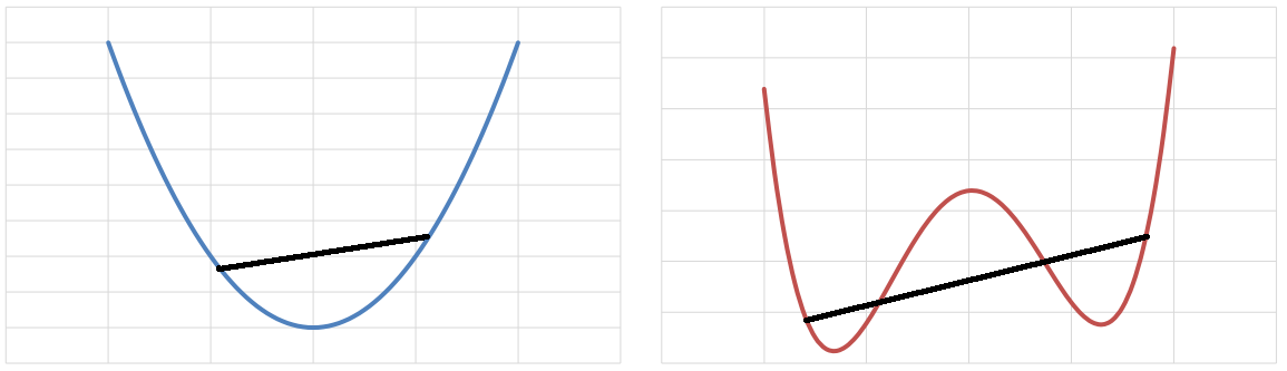
Finding the global minimum of a simple non-convex function such as the one shown in Figure 1 can be achieved relatively easily because of how computationally inexpensive the function is to evaluate, the low dimension, and the low number of local minima. However, ABM-based spatial simulations are often computationally intensive and thus expensive to evaluate, have many parameters resulting in a high-dimensional parameter space, and are vastly complex with a plethora of local minima. More generally, non-convex optimization problems are known to be \(\mathcal{NP}\)-hard while some such problems have even been shown to be \(\mathcal{NP}\)-hard to solve approximately (Jain & Kar 2017). The randomness of ABMs even makes this already difficult optimization even harder as advances in cyberGIS (Wang 2010) and cyberinfrastructure have enabled modelers to create finer-grain, larger-scale, and more complex models.
The difficulty of calibration has led modelers to heavily rely on discretization of their parameter spaces, model reduction, and heuristics. Discretization refers to turning a continuous space with infinitely small granularity into a finite space with coarse granularity. As an example, a parameter \(\alpha \in [0,100]\) might be discretized to \(\alpha \in \{0,10,20,\cdots, 100\}\), yielding a much easier space to search. While discretization can be useful and all computational models must tolerate some level of discretization error, discretization at this level assumes that models are continuous meaning that small changes in each parameter yield only small changes in the model’s outputs. Using a large-grain search of a parameter space also means that the search may miss important optima and equilibria that lie between chosen samples.
Model reduction refers to calibrating a model using a subset of the parameters that best represent the overall performance of the model (Oremland & Laubenbacher 2014). This can be achieved in a variety of ways including global sensitivity analysis (Kang & Aldstadt 2019a; Ligmann-Zielinska et al. 2014) and Cohen’s weighted \(\kappa\) (Oremland & Laubenbacher 2014). While sensitivity analysis is useful for verification of a model (Crooks et al. 2008; Ngo & See 2012), model reduction results in a loss of information and can have unforeseen consequences for ABMs. ABMs often have complex, non-linear relationships between input parameters suggesting that time-saving approaches to optimization such as model reduction and one-at-a-time1 optimization may not be well-suited for ABM calibration.
Using heuristics to solve problems in model calibration requires that we accept solutions that may not be optimal, whether we rely on discretization, model reduction, both, or neither, but it is a sacrifice we are forced to accept because of the complexity of non-convex optimization. In the agent-based modeling context, Monte Carlo (Mao & Bian 2011) and genetic algorithms (Oremland & Laubenbacher 2014) are often used to find approximately optimal parameter sets. However, little work has been done to test the effectiveness of swarm intelligence approaches (Acedo et al. 2018; Alaliyat et al. 2019; He et al. 2022). Particle Swarm Optimization (PSO) is particularly well suited for calibrating spatially-explicity ABMs efficiently because it has been successfully applied to many non-convex problems such parameter-tuning in machine learning, its performance is efficient, and it performs well in noisy (Parsopoulos & Vrahatis 2001) and continuously changing environments (Carlisle & Dozier 2000).
Particle Swarm Optimization
Particle Swarm Optimization (PSO) is an evolutionary algorithm for optimizing non-differentiable, non-linear functions introduced in 1995 for use in neural networks by Kennedy and Eberhart (Eberhart & Kennedy 1995; Kennedy & Eberhart 1995). The method was developed by modeling the social behavior of animals like bird flocks and fish schools (Eberhart & Kennedy 1995; Kennedy & Eberhart 1995). PSO and Genetic Algorithms (GA) are similar in that they are population-based search routines. However, while agents in GA evolve based on Darwinian principles of “survival of the fittest,” PSO is based on communication among a population rather than fittest agents reproducing which has been found to be more efficient in some studies (Panda & Padhy 2008).
The PSO method implemented for this research is based on a standardized PSO algorithm. Bratton & Kennedy (2007) provides the necessary parameters and choices for a general-purpose optimizer, allowing users to provide a search space and a desired number of evaluations (number of particles \(\times\) number of generations), both of which are required for Monte Carlo as well. This standard algorithm allows particles to leave the feasible region, referred to as “letting the particles fly”, but not evaluating them outside of the feasible region to reduce a bias towards the center of the parameter space (Bratton & Kennedy 2007). It also includes a constriction factor \(k\), seen in the Update Step of Figure 2 and Equation 2, which reduces time spent outside of the feasible region and aids in convergence (Bratton & Kennedy 2007; Eberhart & Shi 2000).
The standard algorithm developed by Bratton & Kennedy (2007) recommends methods for initialization that shift the starting positions of the particles away from the global optimum, but notes that for practical optimization applications this strategic initialization is unnecessary. Thus, our PSO algorithm initializes particles uniformly throughout the feasible region and gives particles a random velocity. Once initialized, the algorithm enters an optimization loop as shown in Figure 2. During each iteration of the optimization loop, if particles are within the feasible region, they evaluate their fitness against the cost function using their positions in the parameter space. If the position results in the minimum error achieved by that particle, it is recorded as its individual best or \(\overrightarrow{p}_{b}\). Particles then communicate with their neighbors to determine the minimum position experienced among them which is recorded. When all particles are connected, this is the global best or \(\overrightarrow{g}_{b}\) strategy.
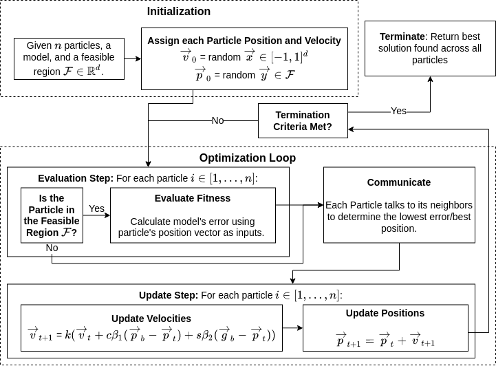
After the evaluation and communication steps of the optimization loop are complete, PSO updates the velocities and positions of the particles as shown in the Update Step of Figure 2. Equation 2 sets the particle’s new velocity (\(\overrightarrow{v}_{t+1}\)) as a combination of its current velocity (\(\overrightarrow{v}_{t}\)), the direction of the particle’s individual best position (\(\overrightarrow{p}_{b}\)), and the direction of the best position reported by all neighbors (\(\overrightarrow{g}_{b}\)). The particle velocity update also includes a constriction factor \(k\) determined by Equation 2 and multiplies the individual best position and global best position by cognitive and social constants respectively \(c\) and \(s\), and two uniformly distributed random variables \(\beta_{1},\beta_{2}\). With velocity calculated, each particle’s position is set to its position plus its velocity.
| \[\begin{aligned} \overrightarrow{v}_{t+1} &= k(\overrightarrow{v}_{t}+c \beta_{1} (\overrightarrow{p}_{b}-\overrightarrow{p}_{t})+s \beta_{2} (\overrightarrow{g}_{b}-\overrightarrow{p}_{t})) \\ \overrightarrow{p}_{t+1} &= \overrightarrow{p}_{t} + \overrightarrow{v}_{t+1} \\ where \; &k = \frac{2}{\lvert 2-\phi-\sqrt{\phi^{2}-4\phi}\rvert}, \: \: \phi=c + s, \phi > 4 \end{aligned}\] | \[(2)\] |
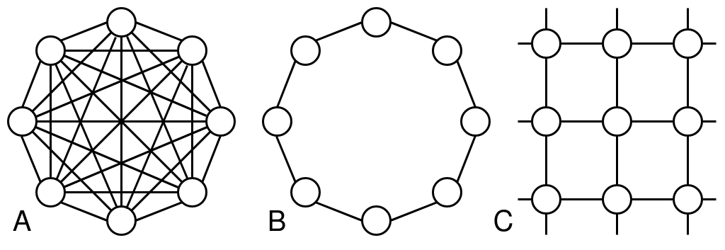
The network structure between the particles allows for information about fitness to propagate through the particles. Choosing a network structure presents a trade-off between convergence and exploration with highly connected networks converging quickly while lowly connected particles are able to explore more (Kennedy & Mendes 2002). While the ring topology is suggested as the standard for PSO by Bratton & Kennedy (2007), they note “that it should not always be considered the optimal choice in all situations”. Thus we have choosen to test three of the most common topologies: fully connected, ring, and a von Neumann network structure. The fully connected version of PSO (Figure 3a) is often referred to as gbest because particles focus on moving towards a global best and is the original version of PSO. The ring topology (Figure 3b) is often referred to as lbest because rather than relying on a global best fitness the particles respond to the best fitness in between itself and its neighbors. Lastly, we chose to test a von Neumann structure (Figuren 3c) because it has been found to be an efficient choice for general-purpose optimization for deterministic functions (Kennedy & Mendes 2002).
The PSO algorithm iterates until it is terminated, which can happen in a variety of ways. The simplest termination criterion is to end the algorithm after a given number of iterations or total evaluations, with the number of iterations being chosen based on the number of parameters and complexity of the space. This is the approach followed by Bratton & Kennedy (2007), Alaliyat et al. (2019) and He et al. (2022). Kwok et al. (2007) and Zielinski & Laur (2007) have discussed a variety of termination criteria including waiting for the particles to be between a short distance of each other, the best fitness to reach a certain point, and the improvement over generations to fall below a threshold. Our implementation has chosen to rely on number of iterations to create a general-purpose solution and reduce the amount of hyper-parameters that have to be tuned.
The PSO algorithm has no dependencies between particles when evaluating fitness at each step, allowing us to evaluate the model concurrently. Our implementation takes advantage of this aspect of the algorithm to exploit parallelism. To speed up our implementation of PSO and better utilize cyberinfrastructure at our disposal, we used the multiprocessing2 package for Python 3.x. In particular, we utilized the Pool class which allows us to create a pool of workers that process particle fitness evaluations. Our code was then run on a multi-node SLURM cluster to ensure it functions well on advanced cyberinfrastructure.
Case Study: ABM of Influenza Transmission
A spatially explicit ABM of influenza transmission in Miami, Florida was used as the case study (Kang et al. 2019). An expanded version of the model has been reported by Kang et al. (2022). It models the spread of influenza throughout a simulated population using a Susceptible-Exposed-Infectious-Recovered (SEIR) model for disease progression. The model was chosen because it is a spatially explicit ABM and the model’s code and associated data have been made available through the CyberGISX platform3 and GitHub4 for computational reproducibility.
The model instantiates heterogeneous human agents based on distributions of age and household size per U.S. Census data. The model utilizes real-world locations of 300 schools, 1,600 workplaces, and 18,000 homes obtained from the Regulatory and Economic Resources Departments Planning Division from Miami-Dade County Open Data Hub.5 Household size and the age of agents are initialized using data from the American Community Survey (ACS). After initialization, we use a distance-based model to assign agents to schools and workplaces: agents between 6 and 19 are assigned to their closest school and agents between 20 to 65 are assigned to their nearest workplace. Agents in the model simulate a typical day: Commuting from school or work and interacting with other agents when they are co-located in households, workplaces, and schools.
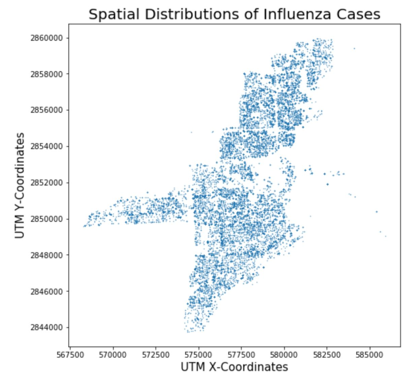
To represent the disease spread process in agents, a SEIR (Susceptible-Exposed-Infectious-Recovered) model was used. The SEIR model is a compartmental model of epidemiology in which agents start off as susceptible to the disease and if they are exposed to the virus they become infectious after an incubation period. A weighted contact network is created from co-location data with weights proportional to the amount of time spent co-located, with school/worked assumed to be 8 hours per day and home assumed to be the rest of the day. Infectious agents can spread influenza to agents they come into contact with until the infectious period ends at which point they become recovered and are assumed to be immune to the virus for the rest of the flu season. A typical result from the model can be seen in Figure 4 which shows the spatial distribution of influenza cases over a flu season.
The ABM contains three parameters: introRate which describes the rate with which human agents are randomly infected with influenza, reproduction which is the expected number of secondary infection cases occurred per an infection case, and infRate which describes the probability that a susceptible person could become exposed when through contact with an infectious person. Approximate ranges for these parameters and the number of days for each step of the SEIR model were informed by the literature on influenza (Ferguson et al. 2006; Heymann 2008; Yang et al. 2009). To measure how well each set of parameters represents real-world influenza transmission trends, we compared the modeling outputs to weekly influenza data obtained from the Florida Department of Health6 as in (Mao 2011) and (Kang & Aldstadt 2019a). The model’s number of infectious agents per week and Florida Health Department influenza cases per week are both normalized. We calculate the absolute error between the two time series to measure the goodness-of-fit of the model (Kang et al. 2019).
Experiments
Our computational experiments are designed to answer two key questions: (1) to what extent can PSO be used to calibrate spatially-explicit ABMs “out-of-the-box” (i.e., without hyperparameter optimization) and (2) how does PSO compare to Monte Carlo in terms of computational efficiency, as measured by the number of evaluations of the model? We used number of evaluations of the model as a metric because neither Monte Carlo or PSO introduces significant overhead. This metric is capable of capturing compute time, memory usage, and I/O and avoids creating a disincentive for exploring parameter sets that may result in longer or more computationally intensive simulation runs. For example, with the model we have chosen, setting introRate to zero will result in no one ever getting infected which results in the model completing much more quickly at the expense of accurately describing the phenomena of interest. We have made the code for both the SEIR model used and the PSO implementation are available on CoMSES: https://www.comses.net/codebase-release/834bd61c-7507-49d3-91d3-85c41564e8f2/.
For all of our experiments, PSO was run with 20 particles with parallel evaluation at each step (as described in Section 3) on the agent-based model of influenza described in Section 4. Bratton & Kennedy (2007) notes that a swarm between 20 and 100 particles gives comparable results and because our search space is only three dimensional we have chosen to use the low end of the range. To test the degree to which PSO’s usefulness relies on hyperparameter settings, we varied the topology and the number of generations, running PSO on the ABM 35 times for each choice of hyperparemter setting. The topologies tested were the fully-connected, ring, and von Neumann (Figure 3). Bratton & Kennedy (2007) do not offer recommendations on the number of iterations, so we turned to the work of Alaliyat et al. (2019) which similarly tuned 3 parameters on a spatially-explicit ABM and chose 50 generations. Thus, for each choice of topology, we ran PSO using 48, 60, and 72 generations to understand how the choice of number of generations affects the performance on PSO’s ability to calibrate the spatially-explicit ABM.
Similarly, we ran Monte Carlo against the model. Rather than generations, Monte Carlo allows us to specify the number of evaluations we would like to take of the model and we chose 500, 750, and 1,000 so that Monte Carlo and PSO would make approximately the same number of evaluations of the model. Just as with the PSO experiments, Monte Carlo was run 35 times on the agent-based model for each choice of 500, 750, and 1,000 evaluations.
For both Monte Carlo and PSO, we measure the goodness-of-fit of the position in the parameter space by running the model with the parameters given by the particle’s position and compute the absolute error between the model’s output and actual case data from the Florida Department of Health. Both the case data and model outputs are normalized before absolute error is calculated so that we can compare infection rates and mitigate errors that may arise from using actual case numbers. The model operates at the granularity of a week to match the granularity of the data from the Florida Department of Health, so absolute error between the model and the case data is calculated at each time step and summed to determine an relative metric for goodness-of-fit. We are interested in the “best” set of parameters each optimization method can find as measured by lowest error and the error of those parameters.
Results
PSO performance
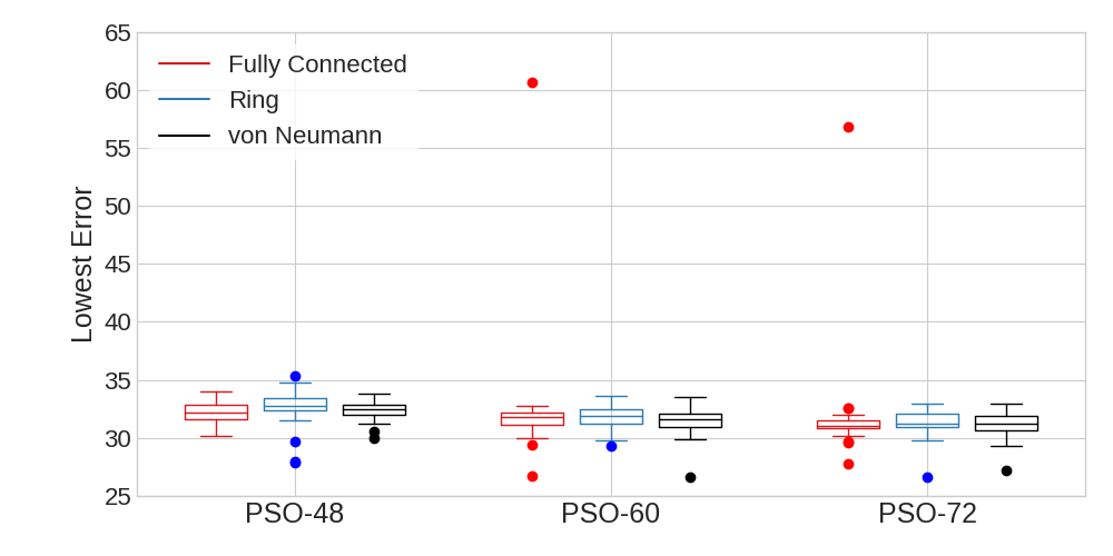
First, we compare how PSO varied across parameter settings. The summary statistics for PSO applied to the spatially-explicit ABM can be seen in Table 1. In Table 1, “Gen” gives the number of generations that PSO was run, “\(\mu\) N Evals”, “\(\sigma\) N Evals” and “CV N Evals” give the mean, standard deviation, and coefficient of variation (\(\sigma/\mu\)) respectively for the number of times the model was evaluated. “Median Err”, “\(\mu\) Err”, “\(\sigma\) Err”, and “CV Err” give the median, mean, standard deviation and coefficient of variation of error achieved across all 35 runs. These measures allow us to quantify the computational cost and performance of each method. The distribution of the lowest error for each run of the PSO experiments is visualized using boxplots in Figure 5.
| Gen | \(\mu\) N Evals | \(\sigma\) N Evals | CV N Evals | Median Err | \(\mu\) Err | \(\sigma\) Err | CV Err | |
|---|---|---|---|---|---|---|---|---|
| Fully Connected | 48 | 440.51 | 51.90 | 11.78% | 32.19 | 32.14 | 0.94 | 2.92% |
| 60 | 660.83 | 57.04 | 8.63% | 31.77 | 32.29 | 5.00 | 15.48% | |
| 72 | 872.34 | 116.36 | 13.34% | 31.06 | 31.75 | 4.38 | 13.80% | |
| Ring | 48 | 418.63 | 30.58 | 7.30% | 32.73 | 32.64 | 1.58 | 4.84% |
| 60 | 608.00 | 36.95 | 6.08% | 31.85 | 31.64 | 1.07 | 3.38% | |
| 72 | 821.20 | 46.96 | 5.72% | 31.23 | 31.31 | 1.16 | 3.70% | |
| von Neumann | 48 | 411.51 | 36.87 | 8.96% | 32.41 | 32.39 | 0.80 | 2.47% |
| 60 | 608.31 | 55.13 | 11.03% | 31.58 | 31.46 | 1.19 | 3.78% | |
| 72 | 833.26 | 54.69 | 6.56% | 31.21 | 31.08 | 1.12 | 3.60% | |
Comparing performance across topologies, the plots in Figure 5 indicate that all of the topologies have comparable performances, however the fully-connected topology appears to be more prone to outliers. The outliers experienced by the fully-connected topology for 60 and 72 generations are also reflected in much larger standard deviations of error in Table 1. These outliers in performance are likely a result of the high connectivity in the topology. Because each particle is connected to every other, the topology sometimes results in the swarm converging on local optima early without adequately exploring the parameter space (Kennedy & Mendes 2002). Despite these occasional outliers for the fully-connected topology, the results show that all three topologies have mean performances that are within a standard deviation of each other for each chosen number of generations. This is an unexpected result given the literature that suggests the Ring (Bratton & Kennedy 2007) and von Neumann (Kennedy & Mendes 2002) tend to outperform the Fully Connected topology but it may be that the stochastic nature of the ABM helped PSO to avoid converging on local minima (Parsopoulos & Vrahatis 2001).
We turn next to examine how the number of generations chosen for PSO affects the performance of the method. Table 1 shows some differences in the performance of PSO as a function of the number of generations, but these differences are not statistically significant, suggesting that “good” results can be obtained regardless of the choice of number of generations. Interestingly, the median error falls as the number of generations increases for each topology suggesting that the algorithm is slightly improving as it goes on. Similarly, we see that the mean error falls slightly as the number of generations rise for the ring and von Neumann topologies, but the outliers cause fully-connected’s mean error to rise between 48 and 60 generations before falling again between 60 and 72 generations. Interestingly, the von Neumann topology is the only one where the standard deviation and coefficient of variance (CV) of error (“\(\sigma\) Err” and “CV Err” in Table 1) fell consistently as the number of generations rose and it would be interesting to see if this pattern would be consistent on more models and across more choices of number of generations.
Turning to the computational efficiency of choices for the number of generations, it is important to note that the number of evaluations does not equal the number of generations times the number of particles because particles are not evaluated during a generation if they lie outside of the bounds. As noted in Section 3, we do not require particles to stay within the bounds of the parameter space because that leads to a bias towards the center of the parameter space (Bratton & Kennedy 2007). To illustrate this, we can see in Table 1 that the increase from 48 to 60 generations is a 25% increase, but for fully-connected this resulted in an approximately 50% increase in the number of evaluations, while the increase from 60 to 72 generations represents a 20% increase, but a 32% increase of evaluations for fully-connected. For a large number of generations, we would expect the increase in generations to match the increase in model evaluations because the particles should converge on a solution and therefore spend more time within the bounds of the parameters.
By analyzing how the number of model evaluations changes as a function of the number of generations, we see that the number of evaluations is roughly the same for each choice of topology. The fully-connected topology uses more evaluations on average for each chosen number of generations, but the differences are not statistically significant. For the ring and von Neumann topologies we see that the standard deviation as a percentage of mean (coefficient of variation) of the number of evaluations (“CV N Evals” in Table 1) declines consistently as the number of generations rises. In contrast, the coefficient of variation increases from 48 generations to 72 generations for the fully-connected topology. Taken together, it appears that the computational efficiency of the ring and von Neumann topologies is more consistent than the fully-connected topology, while differences in the computational efficiency of the topologies are not statistically significant.
From these experiments we are able to observe that PSO’s performance is not greatly affected by the choice of topology and the number of generations. While the performance of fully connected was comparable to that of ring and von Neumann, the latter topologies produce more consistent results. This finding is mirrored in analyzing the computational efficiency of the topologies. Our analysis also shows that while allowing PSO to run over a large number of generations seems to have a positive effect, the results do not change significantly for the number of generations tested. Overall, the findings suggest that our PSO implementation can be applied with confidence “out-of-the-box” to spatially-explicit ABMs without much need for fine-tuning hyperparameter choices like topology and number of generations, although the ring and von Neumann topologies tend to have greater consistency meaning they should be favored by practitioners.
Efficiency compared to Monte Carlo
Although we have demonstrated that PSO’s effectivness is relatively stable across hyperparameter choices and can therefore be used “out-of-the-box”, our fitness metric is a relative one. To contextualize this performance, we used Monte Carlo to evaluate the same ABM with the same parameter ranges. We tested Monte Carlo using 500, 750, and 1000 evaluations respectively so that the number of evaluations is comparable to those used by PSO and ran the algorithm 35 times for each chosen number of evaluations. This helps us to answer the question of how efficient PSO is compared to the commonly-used Monte Carlo method.
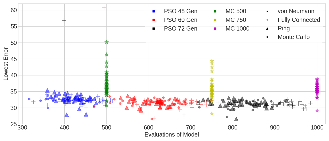
Table 2 gives the summary statistics for the Monte Carlo experiments. Just as in Table 1, “Median Fit”, “\(\mu\) Fit”, “\(\sigma\) Fit”, and “CV Fit” describe the median, mean, standard deviation, and coefficient of variation for the best error found by each run of Monte Carlo. Note that unlike in Table 1, there are no statistics for the number of evaluations because Monte Carlo allows us to specify that explicitly while the PSO method has us specify a number of generations instead. This data is also visualized in Figures 6 and 7 which give boxplots of the performance of the methods and a scatterplot illustrating the performance versus computational efficiency respectively.
| Evals | Median Err | \(\mu\) Err | \(\sigma\) Err | CV Err |
|---|---|---|---|---|
| 500 | 36.88 | 37.46 | 3.93 | 10.49% |
| 750 | 35.63 | 36.07 | 3.09 | 8.57% |
| 1,000 | 35.81 | 35.72 | 1.81 | 5.07% |
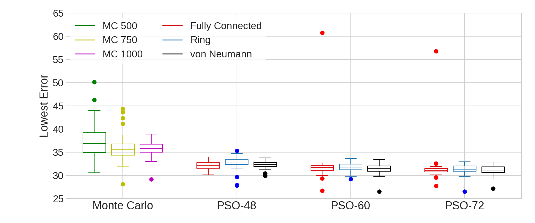
From Tables 1 and 2, we see that PSO’s mean and median minimum errors are below that of Monte Carlo for all PSO and Monte Carlo parameter choices including those where Monte Carlo uses more than twice as many evaluations. The plots in Figure 6 illustrate the drastic difference in the distributions of error with PSO consistently much lower than Monte Carlo. Additionally, while the median error fell as the number of generations grows for each PSO topology, we observe that the median error actually increases for Monte Carlo from 750 to 1,000 evaluations. Interestingly, the mean error fell as the number of evaluations rises for Monte Carlo as well as the ring and von Neumann topologies, but not for the fully-connected topology as a result of the outliers it encountered.
Comparing the consistency of the performance between the two methods, the ring topology’s performance has lower coefficient of variance for every choice of PSO parameters and number of Monte Carlo evaluations. Von Neumann also beats Monte Carlo in consistency except when comparing 48 generations to 1,000 Monte Carlo evaluations where von Neumann still has a lower standard deviation in absolute terms. The fully-connected topology’s outliers mean that despite having better median and mean performance than Monte Carlo, the performance has a higher coefficient of variance, meaning its results are less consistent than Monte Carlo.
Comparing the computational efficiency, Figure 7 gives a plot of the error versus number of evaluations of the model for each experiment. This allows us to visualize the trade-off between performance and computational efficiency. As we would expect, both methods tend to slightly improve as the number of evaluations of the model increase. However, we can see that choosing PSO over Monte Carlo increases our computational efficiency while increasing the quality of our parameters, giving us the best of both worlds.
Overall, it is clear that PSO produces much better parameter sets and is able to do so with lower computational cost than Monte Carlo. PSO was able to achieve a 9.4-20.5% decrease in mean error and an 8.9-18.7% decrease in median error even when PSO used less than half the number of evaluations as Monte Carlo. From these findings, we conclude that PSO not only out-performs Monte Carlo in terms of optimization of spatially-explicit agent-based models, but also does so in a more computationally efficient manner.
Discussion
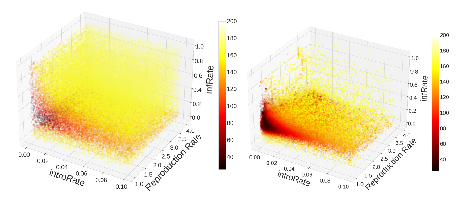
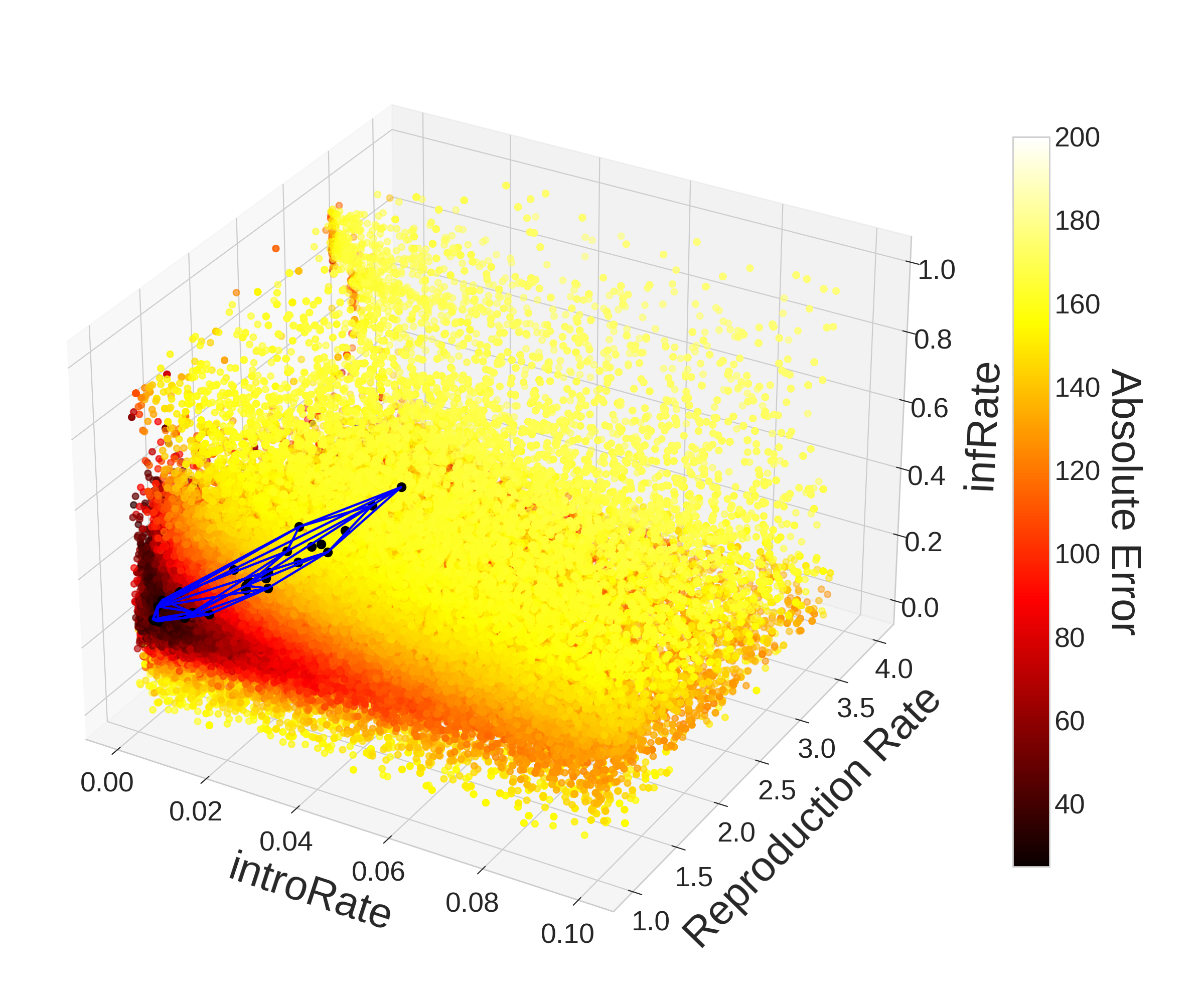
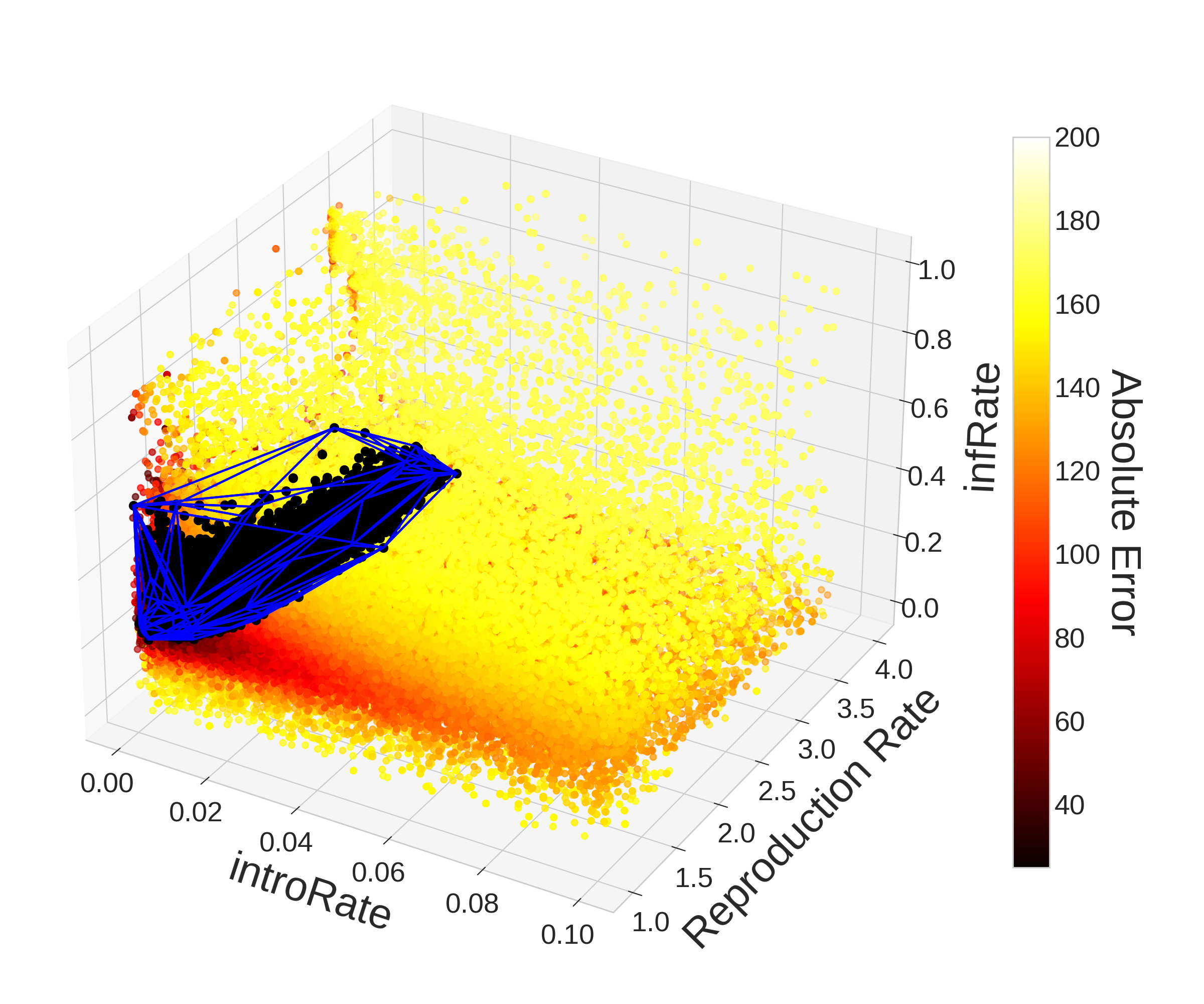
With the benefit of hindsight, we can visualize the parameter space to understand why optimization may be difficult and why PSO was able to outperform Monte Carlo. The left plot in Figure 8 gives us a 3-D visualization of the parameter space with the colorbar indicating the error between the model outputs and observed case data. The visualization was created using the 78,750 points in the parameter space evaluated by Monte Carlo. The Monte Carlo results seem to uniformly cover the 3-D parameter space which is expected as each point is chosen randomly from the parameter space. The specs of darker colors surrounded by yellow represent local minima in the parameter space that could trick traditional optimization methods like gradient descent.
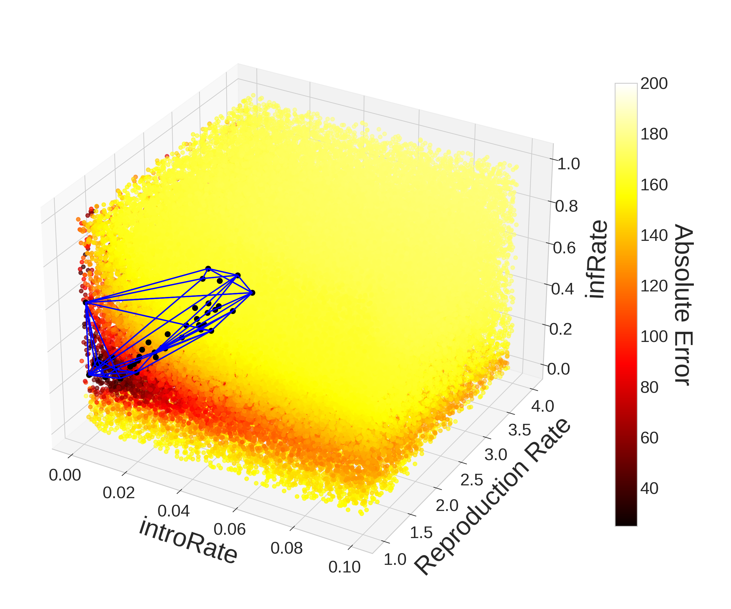
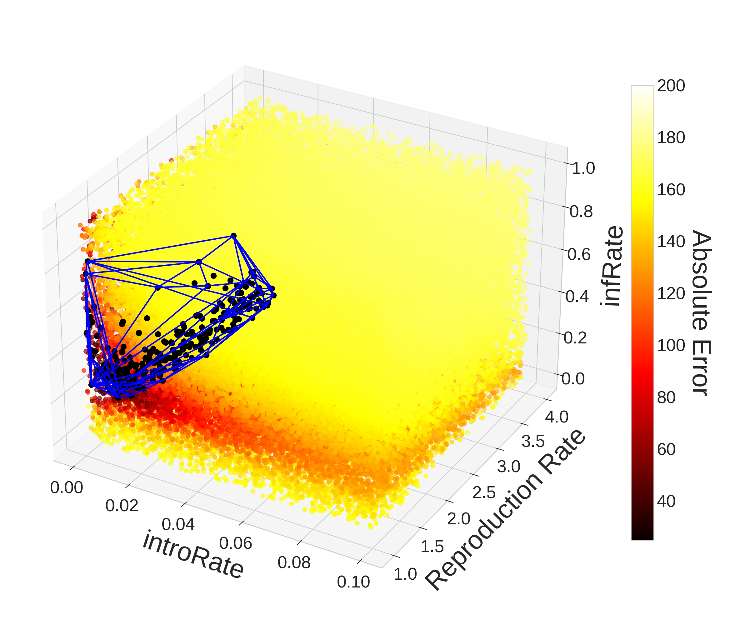
Over the 78,750 evaluations taken by Monte Carlo, only 288 (0.37%) yielded an error below 40. Taking the convex hull of these points, we get an area that represents only about 2.83% of the volume of the parameter space. Narrowing our search to points which yielded an absolute error below 35, we get only 40 (0.05%) points which give us a convex hull that represents 1.17% of the volume of the parameter space. Despite how small these volumes may seem, the stochasticity in the ABM and non-convexity of the error function means that even if a point is within these convex hulls, it may not produce a result that is below the thresholds we used to construct the hulls. In fact these convex hulls contain a total of 2299 (2.92%) and 908 (1.15%) evaluated points respectively despite only 288 and 40 points producing an error below 40 and 35. Therefore only 12.53% and 4.41% of points within the convex hulls respectively fell below the thresholds of 40 and 35 absolute error. Of the 78,750 evaluations, only 2 (0.0025%) yielded a result with error below 30.
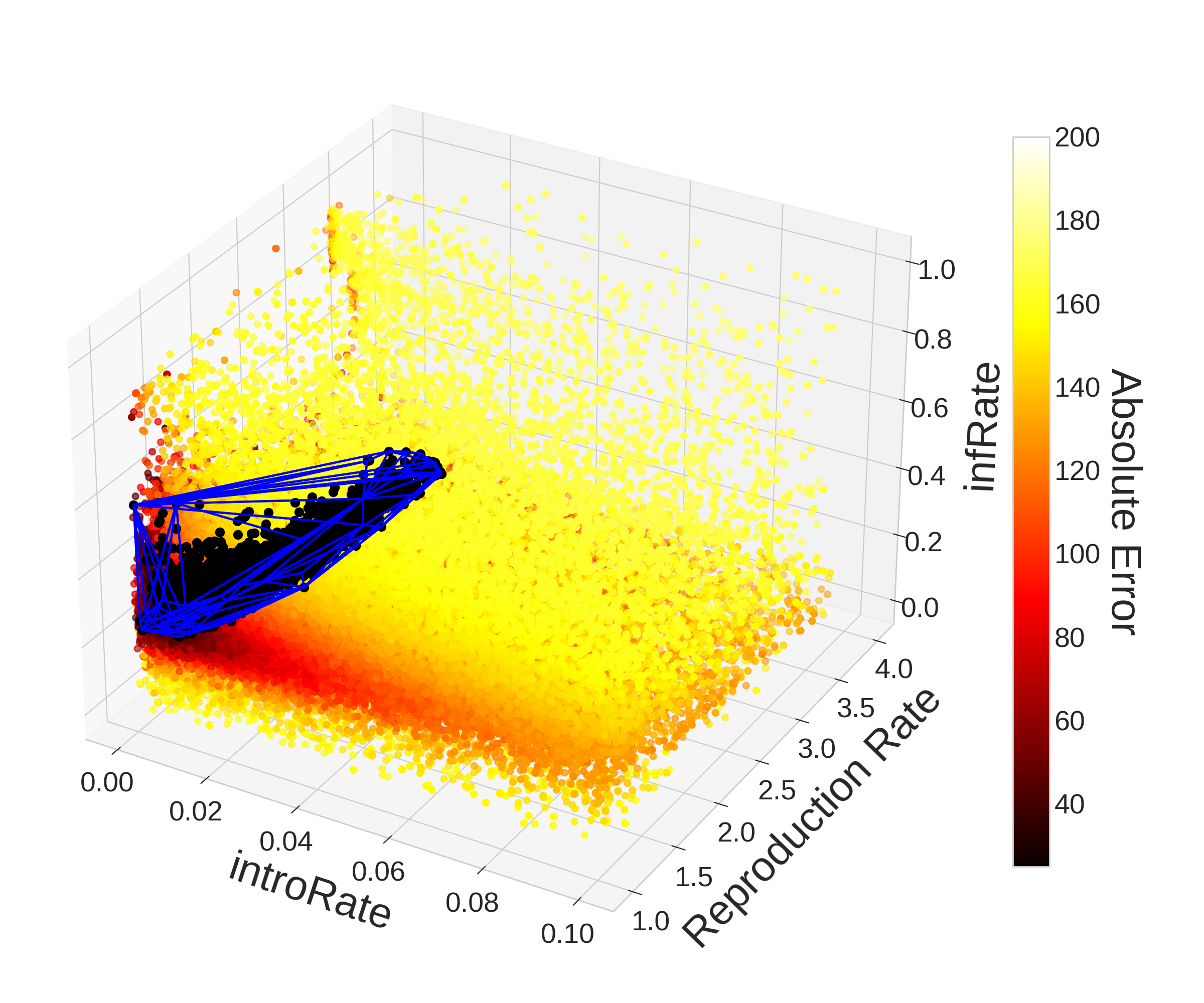
The right plot in Figure 8 was created with the 199,812 evaluations taken using PSO including all hyperparameter choices (topology and number of generations). When comparing the plots in Figure 8, the value of PSO becomes obvious–the region in the upper-right (\([{0.04,0.1}]\times [{1,4}]\times [{0.2,1}]\)) is much less densely population compared to the left plot in Figure 8 despite the figure representing over two and half times more evaluations. This demonstrates the power of PSO’s communication strategy in allowing particles to explore the entire parameter space while focusing more attention on areas that tend to yield better results.
In contrast to Monte Carlo, PSO found 43,915 (22.1%) points that yielded an absolute error below 40 and 7,204 (3.6%) points that yielded an absolute error below 35 representing 60 and 71 times as many points respectively even after adjusting for differences in the total number of evaluations. This significant improvement in performance is explained by the relative amount of evaluations within optimal regions of the parameter space. Compared to Monte Carlo’s 2.92% and 1.15% of evaluations lying within the convex hulls of the points yielding an error of 40 and 35, PSO had 112,779 (56.8%) and 100,608 (50.7%) points within them. So despite only 38.9% and 7.2% of points falling within the convex hulls producing an absolute error below the threshold respectively, the increased time spent in these regions yielded much better parameter sets overall. PSO also found 25 (0.01%) points that produced an error below 30, while Monte Carlo only found 2 (0.0025%). While Monte Carlo’s 2 points do not form a convex hull with volume, the 25 points found by PSO form a convex hull with volume that represents 0.30% of the parameter space. It is worth noting that 40,896 (20.59%) of evaluations were within that region with only 0.06% (25) of them resulted in an error below 30. Full plots of the convex hulls discussed can be viewed in the Appendix.
Conclusions and Future Work
This study demonstrates that PSO can be an efficient method for calibrating ABMs. Specifically, a standard implementation of PSO based on the work by Bratton & Kennedy (2007) can be successfully used out-of-the-box and with a variety of hyperparameter choices, meaning that modelers who choose to adopt PSO will not be held back by a steep learning curve. Our results show comparable performance for all three choices of topology and number of generations, with all hyperparameter choices outperforming Monte Carlo. Furthermore, our PSO approach is able to produce better parameter sets than Monte Carlo while achieving higher computational efficiency. Our computational experiments suggest that the ring and von Neumann topologies should be favored over the fully-connected topology for greater consistency.
There are a number of potential improvements that could be made to the PSO algorithm described in this paper. Our implementation initialized particle position using uniformly random distribution in the bounds of the parameter space to match Monte Carlo’s selection process, but work has shown that using low-discrepancy quasi-random sequences can improve performance (Pant et al. 2008). Although we have tested the network structures the literature recommends, there are network communication structures beyond the three explored including random networks (Kennedy 1999), “pyramid”, and “star” (Kennedy & Mendes 2002) which may lend themselves better to optimizing ABMs. While we have chosen a standardized implementation for this study, there are many variations on the algorithm which may be even better suited for calibrating ABMs (Banks et al. 2007; Carlisle & Dozier 2000). As discussed in Section 3, there are also a variety of metrics to determine when the PSO algorithm should terminate, which can be further explored on a wider set of ABMs. Poli et al. (2007) gives an overview of the variations and open questions surrounding PSO which will be helpful for future work in this direction.
Further experimentation is needed to determine if PSO is effective and efficient on a wider variety of ABMs. In particular, it is important to understand how PSO compares to other optimization methods as the number of model parameters and complexity increase. Further work is also needed to compare how PSO’s performance and efficiency compare to other heuristic optimization methods and techniques that rely on model reduction. While Parsopoulos & Vrahatis (2001) suggests that PSO performs well under noisy and continuously changing environments, it would be informative to explore how this standardized PSO performs for dynamic calibration of a model as new interventions occur. The PySwarm Python package by Miranda (2018) and the approach described in this paper offer great potential for further exploration. Beyond Particle Swarm Optimization, there are other interesting swarm intelligence algorithms which could be explored such as Artificial Bee Colony (ABC) optimization (Karaboga & Basturk 2007).
Acknowledgements
This material is based upon work supported by the Institute for Geospatial Understanding through an Integrative Discovery Environment (I-GUIDE) that is supported by the National Science Foundation (NSF) under award No. 2118329. The material is also based in part upon work supported by NSF under grant No. 1824961. Any opinions, findings, and conclusions or recommendations expressed in this material are those of the authors and do not necessarily reflect the views of NSF. Our computational work used Virtual ROGER, which is a cyberGIS supercomputer supported by the CyberGIS center for Advanced Digital and Spatial Studies and the School of Earth, Society and Environment at the University of Illinois Urbana-Champaign.Notes
where one parameter is varied while the others remain the same↩︎
The model can be accessed and executed on the CyberGISX environment: https://cybergisxhub.cigi.illinois.edu/notebook/a-reproducible-and-replicable-spatially-explicit-agent-based-model-using-cybergis-jupyter-a-case-study-in-queen-anne-neighborhood-seattle-wa/↩︎
The Github repository for the ABM can be found at https://github.com/cybergis/QueenAnneFlu↩︎
Miami-Dade County Open Data Hub: http://gis-mdc.opendata.arcgis.com/↩︎
Florida Department of Health Influenza Data: http://www.floridahealth.gov/diseases-and-conditions/influenza/florida-influenza-surveillance-report-archive↩︎
Appendix: Convex Hull Plots
References
ACEDO, L., Burgos, C., Hidalgo, J.-I., Sánchez-Alonso, V., Villanueva, R. J., & Villanueva-Oller, J. (2018). Calibrating a large network model describing the transmission dynamics of the human papillomavirus using a particle swarm optimization algorithm in a distributed computing environment. The International Journal of High Performance Computing Applications, 32(5), 721–728. [doi:10.1177/1094342017697862]
ALALIYAT, S., Yndestad, H., & Davidsen, P. I. (2019). Optimal fish densities and farm locations in Norwegian fjords: A framework to use a PSO algorithm to optimize an agent-based model to simulate fish disease dynamics. Aquaculture International, 27(3), 747–770. [doi:10.1007/s10499-019-00366-6]
BANKS, A., Vincent, J., & Anyakoha, C. (2007). A review of particle swarm optimization. Part I: Background and development. Natural Computing, 6(4), 467–484. [doi:10.1007/s11047-007-9049-5]
BRATTON, D., & Kennedy, J. (2007). Defining a standard for particle swarm optimization. 2007 IEEE Swarm Intellinge Symposium. Available at: https://ieeexplore.ieee.org/document/4223164. [doi:10.1109/sis.2007.368035]
CARLISLE, A., & Dozier, G. (2000). Adapting particle swarm optimization to dynamic environments. Proceedings, 2000 ICAI, Las Vegas, NV. Available at: http://citeseerx.ist.psu.edu/viewdoc/download?doi=101.1.589.895&rep=rep1&type=pdf.
CLARKE, K. (2018). 'Land use change modeling with sleuth: Improving calibration with a genetic algorithm.' In M. T. Camacho Olmedo, M. Paegelow, J. F. Mas, & F. Escobar (Eds.), Geomatic Approaches for Modeling Land Change Scenarios (pp. 139–161). Berlin Heidelberg: Springer. [doi:10.1007/978-3-319-60801-3_8]
CROOKS, A., Castle, C., & Batty, M. (2008). Key challenges in agent-based modelling for geo-spatial simulation. Computers, Environment and Urban Systems, 32(6), 417–430. [doi:10.1016/j.compenvurbsys.2008.09.004]
EBERHART, R., & Kennedy, J. (1995). A new optimizer using particle Swarm theory. MHS’95. Proceedings of the Sixth International Symposium on Micro Machine and Human Science. [doi:10.1109/mhs.1995.494215]
EBERHART, R., & Shi, Y. (2000). Comparing inertia weights and constriction factors in particle swarm optimization. Proceedings of the 2000 Congress on Evolutionary Computation. Available at: https://ieeexplore.ieee.org/document/870279. [doi:10.1109/cec.2000.870279]
FERGUSON, N. M., Cummings, D. A. T., Fraser, C., Cajka, J. C., Cooley, P. C., & Burke, D. S. (2006). Strategies for mitigating an influenza pandemic. Nature, 442(7101), 448–452. [doi:10.1038/nature04795]
FILATOVA, T., Parker, D., & van der Veen, A. (2009). Agent-Based urban land markets: Agent’s pricing behavior, land prices and urban land use change. Journal of Artificial Societies and Social Simulation, 12(1), 3: https://www.jasss.org/12/1/3.html.
GRIMM, V., Revilla, E., Berger, U., Jeltsch, F., Mooij, W. M., Railsback, S. F., Thulke, H.-H., Weiner, J., Wiegand, T., & DeAngelis, D. L. (2005). Pattern-Oriented modeling of agent-Based complex systems: Lessons from ecology. Science, 310(5750), 987–991. [doi:10.1126/science.1116681]
HE, H., Buchholtz, E., Chen, F., Vogel, S., & Yu, C. A. (. (2022). An agent-based model of elephant crop consumption walks using combinatorial optimization. Ecological Modelling, 464, 109852. [doi:10.1016/j.ecolmodel.2021.109852]
HEYMANN, D. L. (2008). Control of Communicable Diseases Manual. Oxford: Oxford University Press.
JAIN, P., & Kar, P. (2017). Non-Convex Optimization for Machine Learning. Boston, MA: Now Foundations; Trends.
KANG, J. Y., & Aldstadt, J. (2019a). Using multiple scale space-time patterns in variance-based global sensitivity analysis for spatially explicit agent-based models. Computers, Environment and Urban Systems, 75, 170–183. [doi:10.1016/j.compenvurbsys.2019.02.006]
KANG, J. Y., & Aldstadt, J. (2019b). Using multiple scale spatio-temporal patterns for validating spatially explicit agent-based models. International Journal of Geographical Information Science, 33(1), 193–213. [doi:10.1080/13658816.2018.1535121]
KANG, J.-Y., Aldstadt, J., Michels, A., Vandewalle, R., & Wang, S. (2019). CyberGIS-Jupyter for spatially explicit agent-Based modeling: A case study on influenza transmission. Proceedings of the 2nd ACM SIGSPATIAL International Workshop on GeoSpatial Simulation, Chicago, Illinois. Available at: https://dl.acm.org/doi/10.1145/3356470.3365531. [doi:10.1145/3356470.3365531]
KANG, J. Y., Aldstadt, J., Vandewalle, R., Yin, D., & Wang, S. (2020). A CyberGIS approach to spatiotemporally explicit uncertainty and global sensitivity analysis for agent-Based modeling of vector-Borne disease transmission. Annals of the American Association of Geographers, 110(6), 1855–1873. [doi:10.1080/24694452.2020.1723400]
KANG, J. Y., Michels, A., Crooks, A., Aldstadt, J., & Wang, S. (2022). An integrated framework of global sensitivity analysis and calibration for spatially explicit agent-based models. Transactions in GIS, 26(1), 100–128. [doi:10.1111/tgis.12837]
KARABOGA, D., & Basturk, B. (2007). A powerful and efficient algorithm for numerical function optimization: Artificial Bee Colony (ABC) algorithm. Journal of Global Optimization, 39(3), 459–471. [doi:10.1007/s10898-007-9149-x]
KENNEDY, J. (1999). Small worlds and mega-minds: Effects of neighborhood topology on particle swarm performance. Proceedings of the 1999 Congress on Evolutionary Computation-CEC99. Available at: https://ieeexplore.ieee.org/document/785509. [doi:10.1109/cec.1999.785509]
KENNEDY, J., & Eberhart, R. (1995). Particle swarm optimization. Proceedings of ICNN’95 - International Conference on Neural Networks. Available at: https://ieeexplore.ieee.org/document/488968. [doi:10.1109/icnn.1995.488968]
KENNEDY, J., & Mendes, R. (2002). Population structure and particle swarm performance. Proceedings of the 2002 Congress on Evolutionary Computation. Available at: https://ieeexplore.ieee.org/document/1004493. [doi:10.1109/cec.2002.1004493]
KWOK, N. M., Ha, Q. P., Liu, D. K., Fang, G., & Tan, K. C. (2007). Efficient particle swarm optimization: A termination condition based on the decision-making approach. 2007 IEEE Congress on Evolutionary Computation. Available at: https://ieeexplore.ieee.org/document/4424905. [doi:10.1109/cec.2007.4424905]
LIGMANN-ZIELINSKA, A., Kramer, D. B., Spence Cheruvelil, K., & Soranno, P. A. (2014). Using uncertainty and sensitivity analyses in socioecological agent-Based models to improve their analytical performance and policy relevance. PLoS ONE, 9(10), 1–13. [doi:10.1371/journal.pone.0109779]
LIU, Z., Rexachs, D., Epelde, F., & Luque, E. (2017). A simulation and optimization based method for calibrating agent-based emergency department models under data scarcity. Computers & Industrial Engineering, 103, 300–309. [doi:10.1016/j.cie.2016.11.036]
MANSON, S., An, L., Clarke, K. C., Heppenstall, A., Koch, J., Krzyzanowski, B., Morgan, F., O’Sullivan, D., Runck, B. C., Shook, E., & Tesfatsion, L. (2020). Methodological issues of spatial agent-based models. Journal of Artificial Societies and Social Simulation, 23(1), 3: https://www.jasss.org/23/1/3.html. [doi:10.18564/jasss.4174]
MAO, L. (2011). Agent-based simulation for weekend-extension strategies to mitigate influenza outbreaks. BMC Public Health, 11(1), 522. [doi:10.1186/1471-2458-11-522]
MAO, L., & Bian, L. (2011). Agent-based simulation for a dual-diffusion process of influenza and human preventive behavior. International Journal of Geographical Information Science, 25(9), 1371–1388. [doi:10.1080/13658816.2011.556121]
MIRANDA, L. J. (2018). PySwarms: A research toolkit for particle swarm optimization in Python. Journal of Open Source Software, 3(21), 433.
NGO, T. A., & See, L. (2012). 'Calibration and validation of agent-Based models of land cover change.' In A. J. Heppenstall, A. T. Crooks, L. M. See, & M. Batty (Eds.), Agent-Based Models of Geographical Systems (pp. 181–197). Berlin Heidelberg: Springer Netherlands. [doi:10.1007/978-90-481-8927-4_10]
OREMLAND, M., & Laubenbacher, R. (2014). Optimization of agent-Based models: Scaling methods and heuristic algorithms. Journal of Artificial Societies and Social Simulation, 17(2), 6: https://www.jasss.org/17/2/6.html. [doi:10.18564/jasss.2472]
PANDA, S., & Padhy, N. P. (2008). Comparison of particle swarm optimization and genetic algorithm for FACTS-based controller design. Applied Soft Computing, 8(4), 1418–1427. [doi:10.1016/j.asoc.2007.10.009]
PANT, M., Thangaraj, R., Grosan, C., & Abraham, A. (2008). Improved particle swarm optimization with low-discrepancy sequences. 2008 IEEE Congress on Evolutionary Computation (Ieee World Congress on Computational Intelligence), 3011–3018. [doi:10.1109/cec.2008.4631204]
PARSOPOULOS, K., & Vrahatis, M. (2001). Particle swarm optimizer in noisy and continuously changing environments. In M. H. Hamza (Ed.), Artificial intelligence and soft computing (pp. 289–294). Anaheim, CA: IASTED/ACTA Press.
POLI, R., Kennedy, J., & Blackwell, T. (2007). Particle swarm optimization. Swarm Intelligence, 1(1), 33–57. [doi:10.1007/s11721-007-0002-0]
RAIMBAULT, J., Cottineau, C., Le Texier, M., Le Nechet, F., & Reuillon, R. (2019). Space matters: Extending sensitivity analysis to initial spatial conditions in geosimulation models. Journal of Artificial Societies and Social Simulation, 22(4), 10: https://www.jasss.org/22/4/10.html. [doi:10.18564/jasss.4136]
WANG, S. (2010). A cyberGIS framework for the synthesis of Cyberinfrastructure, GIS, and spatial analysis. Annals of the Association of American Geographers, 100(3), 535–557. [doi:10.1080/00045601003791243]
WISE, S. C., & Cheng, T. (2016). How officers create guardianship: An agent-based model of policing. Transactions in GIS, 20(5), 790–806. [doi:10.1111/tgis.12173]
YANG, Y., Sugimoto, J. D., Halloran, M. E., Basta, N. E., Chao, D. L., Matrajt, L., Potter, G., Kenah, E., & Ira M. Longini, J. (2009). The transmissibility and control of pandemic Influenza A (H1N1) virus. Science, 326(5953), 729–733. [doi:10.1126/science.1177373]
ZIELINSKI, K., & Laur, R. (2007). Stopping criteria for a constrained single-objective particle swarm optimization algorithm. Informatica, 31(1), 51–59. [doi:10.1109/cec.2006.1688343]