Methods That Support the Validation of Agent-Based Models: An Overview and Discussion

,
and
aOld Dominion University, United States; bThe MITRE Corporation, United States; cVirginia Modeling, Analysis, and Simulation Center at Old Dominion University, United States
Journal of Artificial
Societies and Social Simulation 27 (1) 11
<https://www.jasss.org/27/1/11.html>
DOI: 10.18564/jasss.5258
Received: 06-Jun-2022 Accepted: 10-Oct-2023 Published: 31-Jan-2024
Abstract
Validation is the process of determining if a model adequately represents the system under study for the model’s intended purpose. Validation is a critical component in building the credibility of a simulation model with its end-users. Effectively conducting validation can be a daunting task for both novice and experienced simulation developers. Further compounding the difficult task of conducting validation is that there is no universally accepted approach for assessing a simulation. These challenges are particularly relevant to the paradigm of Agent-Based Modeling and Simulation (ABMS) because of the complexity found in these models’ mechanisms and in the real-world situations they attempt to represent. To aid both the novice and expert in conducting a validation process for an agent-based simulation, this article reviews nine methods that are useful for this process, including foundational topics of docking, empirical validation, sampling, and visualization, as well as advanced topics of bootstrapping, causal analysis, inverse generative social science, and role-playing. Each method is reviewed with respect to its benefits and limitations as a validation-supporting method for ABMS. Suggestions that may support a validation plan for an agent-based simulations, are also provided. This article is an introductory guide for understanding and conducting ABMS validation for developers of all experience levels.Introduction
Validation is a critical component for building the credibility that a simulation model adequately meets its intended purpose (Law 2015; Naylor & Finger 1967). Credibility is the quality of inspiring belief in the correctness of something. When users and stakeholders can trust that the simulation was diligently and adequately constructed so it addresses the model’s purpose, then credibility grows. Credibility is a ternary relationship between the simulation, the end user, and the systems under study. The relationship is ternary because (i) the stakeholder uses their understanding of the system under study to see if the simulation adequately fits that understanding, (ii) this understanding is, hopefully, informed by the actual system under study, and (iii) the simulation developer uses, hopefully, the system under study to inform the development of the simulation. With this in mind, validation is defined as the process of determining if a model adequately represents the system under study for the model’s intended purpose (Erdemir et al. 2020; Grimm et al. 2020; Sargent & Balci 2017); this definition could be simplified further as building the right model (Balci 1998). What some of the validation-supporting methods are and how they could be practically implemented is the focus of this article. This focus is intended to provide readers with guidance and insight to help them select the validation-supporting methods for use in their validation plan.
Within agent-based modeling, the selection of validation-supporting methods is not a straightforward task because there is no one-size-fits-all approach to validation, nor are there any consistent validation standards that are applicable and/or acceptable across the whole agent-based modeling community (Collins et al. 2015). There might be some fields that use Agent-based Modeling and Simulation (ABMS) that have universally agreed upon validation approach, though the authors where unable to find any. This, coupled with the ever-expanding plethora of new verification and validation-supporting methods being developed (e.g., Collins et al. 2022a; Borgonovo et al. 2022) means that it has become more difficult for a simulation novice to navigate the simulation validation literature. This article aims to help navigate the ever-expanding range of validation-supporting methods suggested for ABMS through a detailed discussion of nine methods and practical guidance for implementation. This article has been written in a discipline-agnostic manner, though it is impossible to mitigate all biases.
Agent-based modeling is conducted in various disciplines, each with its own validation and communication requirements. This can result in differing, sometimes contradictory, advice on how to approach validation. Though this article does not resolve those differences, it is hoped to provide a starting point for a simulation development novice in understanding the validation-supporting methods and approaches available in ABMS.
This article first discusses simulation validation in more detail to give a reader a better understanding of its origin and a few of the controversies. A selected variety of validation-supporting methods are then described. This description is followed by a general discussion on how to select validation-supporting methods. The article concludes with curated recommendations for simulation developers.
Background
In this section, some background is provided, and a little history of validation in the context of modeling and simulation (M&S) in general, then, specifically, agent-based modeling and simulation (ABMS). The focus of this article is validation-supporting methods that can be applied to M&S, specifically ABMS; as such, other forms for validation are not considered. For example, psychologists tend to consider four types of validation in their experiments- internal, external, construction, and statistical (Jhangiani et al. 2015) – which are not discussed in this article.
ABMS is one of several paradigms available in the M&S domain (Law 2015). The M&S community has a sixty-year history (Collins et al. 2022a), which was originally focused on Discrete Event Simulation (DES). Most validation-supporting methods developed by this community were developed for DES (Banks 1998), and some have argued that ABMS is just a subset of DES (Law 2015), so DES validation processes apply to ABMS. However, as the ABMS community diverges from the DES community, so do its applicable validation approaches. This article focuses on validation processes that have been advocated for ABMS.
Note that validation is sometimes used in conjunction with the word verification. Verification is the process of determining if a model is consistent with its specification (Petty 2010). This article focuses on validation, though verification is mentioned at certain points.
Validation of modeling and simulation
The use of multiple definitions is common in the simulation community; for example, Ören (2011) found 400 different definitions of the word “simulation.” In this article, a model is defined as a representation of a system for some intended purpose and a simulation as the dynamic implementation of that model. Inconsistencies in the definitions of terminology can contribute to misinterpretation of outcomes and can result in communication confusion (Barnes III & Konia 2018; David 2006; Glasow & Pace 1999; Roache 1998); however, this article is not intended to be impeded by the semantics of definitions and will thus use the simple definition of validation given in the introduction.
Our definition of validation is, by far, not the only definition of validation that exists. Other definitions include words like “accurate” (Law 2015; Sargent 2013; Schlesinger et al. 1979), “simuland” (Petty 2010), “testability” (Carley 2017), or even “real world” (Department of Defense 2009). These definitions have not been included here to avoid confusion, and the authors will leave the discussion of comparing definitions to a future paper.
The discussion of validation in a simulation context has more than fifty years of history (Sargent & Balci 2017), starting with the first major paper on the topic by Naylor & Finger (1967). This was followed by Fishman & Kiviat (1968), whose work was on a statistical validation approach for discrete-event simulation (DES), which was the emerging simulation paradigm at that time (Collins et al. 2022b). DES is a simulation paradigm that views a dynamic system as a sequence of discrete events, which is a convenient way to simulate as it is analogous to how, pre-parallelization, programs are executed on a computer (i.e., the use of the stack). Until the turn of the century, validation-supporting methods relating to DES dominated the simulation community, with Osman Balci and Robert Sargent being the lead academics in Verification and Validation (V&V) at that time (Sargent & Balci 2017). In a seminal piece of work, Balci identified 75 verification and validation (V&V) techniques (Balci 1998), and that number continues to grow, with new ones being created annually (e.g., Collins et al. 2022a; Borgonovo et al. 2022).
The simulation community has dramatically expanded over the last 30 years, mainly due to advances in personal computers (Collins et al. 2022b; Lynch et al. 2020). As a result, many in the simulation community have never heard of DES, let alone its validation. For example, the Augusiak et al. (2014) review of validation-supporting methods for ecological simulations does not even mention Osman Balci’s work. As such, it is not surprising to expect some development of ABMS validation to occur without this background in DES knowledge. The authors of this article all come from a traditional M&S / system engineering background, which means they are experienced in DES literature, and, as a result, this article might contain biases toward that knowledge base.
Validation process for agent-based modeling and simulation
ABMS is a form of M&S that focuses on the agent paradigm; that is, agents and their behavior form the foundations of the model (North & Macal 2007). Unsurprisingly, there is no universally agreed-upon definition of ABMS across all its communities (Macal 2016). The intent of agent-based modeling is to gain insight into the emergent macro-level behaviors that are observed from interacting heterogeneous agents without the use of aggregation modeling (Epstein 2007; Miller & Page 2007). It is these agents and behaviors that tend to be the focus of validation exercises relating to ABMS.
Some view ABMS as just a subset of DES (Law 2015) because it is implemented on a computer using discrete events, and, as such, they believe that all DES validation-supporting methods are appropriate. This is not a view shared by all, including the authors, and, as such, different validation-supporting methods have been proposed. This article discusses nine of these approaches (data analytics, docking, empirical validation, sampling, visualization, bootstrapping, causal analysis, inverse generative social science, and role-playing).
The aforementioned techniques are not an exhaustive list, with other methods having been suggested. For example, Heath et al. (2012) advocated the use of unified modeling language (UML) type approaches; Bianchi et al. (2007) applied ex-post experiments as their validation-supporting method; and Carley (2017) talks about testability. Some even advocate for using multiple methods (Klügl 2008; McCourt et al. 2012; Niazi 2011), which is discussed below.
The different validation-supporting methods have been developed by researchers from a variety of academic disciplines. The multidisciplinary nature of ABMS raises the question of whether the different suggested validation-supporting methods are unique or entirely distinct from each other. Different disciplines have different expectations, terminology, theoretical frameworks, and ontologies, which can make it challenging to translate from one academic discipline to another. More importantly, all disciplines have their own biases, and the discipline’s community may not even realize or may trivialize these biases (perhaps due to their epistemic bubbles, Magnani & Bertolotti (2011)). These multidisciplinary differences result in different expectations for a validation process. As such, it is important to consider the intended audience (and their discipline) when choosing validation-supporting methods (this point will be expanded upon in the Discussion section).
These differences in the disciplines even result in different viewpoints on the simulation validation processes. Different definitions of validation for ABMS are being defined for different disciplines: engineering (North & Macal 2007), social sciences (Ormerod & Rosewell 2009), ecology (Railsback & Grimm 2019), and computer science (Wilensky & Rand 2015). As such, the above definition of validation for use with ABMS is retained for simplicity’s sake. This definition is hoped to be discipline-agnostic enough to be useful to the reader.
Given the issue of multidisciplinary interpretation of validation, there is no universal standard method for the ABMS validation process. Given the subjective nature of validation’s definition and its purpose, it is not surprising that there is not one universal validation approach, and the authors would recommend skepticism towards anyone who claims they have developed one. Part of this article’s purpose is to expose the reader to different validation-supporting methods and techniques that might be appropriate for their simulation projects. As Gilbert (2020) stated, “the theory and practice of validation is more complicated and more controversial than one might at first expect”. This article is hoped to provide some guidance in handling these subjective aspects of validation.
Validation-Supporting Methods
A selection of nine validation-supporting methods is presented in this section to provide an understanding of the variety available. Other validation-supporting methods exist, for example, face validation (Balci 1998) and the others mentioned above. The selection of methods was deliberately made from various academic disciplines that use ABMS in an attempt to be inclusive of the whole enterprise that is ABMS. In all nine methods discussed, the focus is placed on a particular instance of the method, e.g., Latin Hyper-cube Sampling, as an example of sampling.
It is an intimidating task for a simulation developer to select a validation-supporting method that is appropriate for their simulation; thus, the nine methods described in this section were chosen to provide an insight into a variety of different approaches and, to further this insight, discussion on the benefits and limitations of each validation-supporting method is provided. Further guidance is provided in the Discussion section.
The methods are split into foundational (data analytics, docking, empirical, sampling, and visualization) and advanced (bootstrapping, causal analysis, iGSS, and role-playing). “Foundational” is defined as those methods that the authors would expect every agent-based modeling expert to know. A detailed description of each of the five foundational methods is given before a more general discussion is given on the four more advanced methods.
Data analytics
Data Analytics is the holistic study of empirical data, including data mining, data management, statistics, and machine learning (Leathrum et al. 2020). This definition is not universal, and other terms are used interchangeably with data analytics, i.e., data science, data analysis, etc. The key feature of data analytics is that it considers the holistic management and use of data, whereas statistical analysis focuses only on the statistical technique or test. Data analytics is important for any simulation development project because handling data, both input and output, can require intense effort (Skoogh & Johansson 2007); thus, deciding which data handling methods are used is worthy of pre-consideration as opposed to ad-hoc decisions.
Data analytic methods provide a means to clean and organize the input and output data for a simulation. This supports the validation process of a simulation because it helps provide transparency toward data collection, management, and application (Lynch et al. 2021). Data analytics also provides a mechanism for input modeling and data modeling: it helps derive the statistical distributions used in the input modeling as well as provides relational structures of data for the data modeling. Input modeling connects data to the probabilistic mechanisms within the simulation. This is important because input data contributes to deriving system structure, input parameters, and modeling assumptions. Unstructured messy data can induce biased structures and unequal variance estimates in differing regions of the sample space.
Given the ever-increasing volumes of available data, it is essential to follow a data management protocol and for the effort to implement a formal data management program. Formal data management programs should preserve and secure original data sets, intermediate structured and cleaned data sets, and output data. This is not to imply that all data must be saved. Simulation development is usually an iterative process: running the simulation, analyzing the output data, changing the simulation, running it again, and so on. Data developed during these “development runs” can often be discarded. When simulation development has ended, then it is time to begin carefully dealing with input and output data used for, and created by, these “runs of record.”
Once a data management protocol has been developed, data wrangling can begin. Data wrangling is data cleaning, which includes gathering, selecting, and transforming data. Data wrangling the simulation input data both reduces the need for complexity and the number of errors made during development (Kavak et al. 2018). This can be further supported by data mining, which is the use of computational algorithms to illuminate meaning, relationships, and patterns. While data mining can highlight subtle patterns in the data and complex relationships among input and output data, many insights can often be generated via simpler methods such as descriptive and sampling statistics. Your choice of data analytics methods should be driven by the questions being asked and should be no more complex than necessary.
Leathrum et al. (2020) describe how data analytics fits into the M&S development process, which Lynch et al. (2021) take and specifically shows how data analytics fits into the validation process. Data analytics formalizes data usage and representation, shows the organization of the data, and builds credibility.
To understand how data analytics could be used in validation, a simplified example from the study of pseudo-random number generators (RNG) is used. The reason for picking this example is that its goal is simple to understand: generate sufficiently random numbers from a seed that is reproducible. There are a variety of tests that can be conducted on a set of data to determine its “randomness,” e.g., run-up test, spectral tests, etc. (Law 2015). Through data exploration, a popular RNG by IBM, known as RANDU, was discovered to have a flaw in that the randomly generated numbers fall into planes, as shown below. In fact, all linear congruential generators (LCG), a form of RNG, suffer from this problem to some degree (Marsaglia 1968).
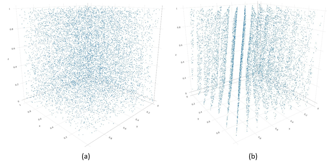
The point here is that the invalidation of RANDU was discovered through the exploration of its generated data. Data analytics provides an approach to conducting this exploration. Simply put, it provides a means to explore the data collected or generated by the simulation to help discover any anomalies.
Benefits and limitations of data analytics
There are many benefits to data analytics as a method to support validation. Obviously, it helps provide a means for the developer to manage and understand their datasets; this provides a deeper understanding of the simuland (i.e., the real-world system under study), which, is hoped, results in a better simulation being built. Looking at the actual data and its resultant logical implications might help remove some of the developers’ unfounded biases that they have about the system. Since data analytics can be used on not only the simulation input data but also its output data and any data used in its validation process, it provides credibility between the validation process and the simulation’s stakeholders by demonstrating that the data was handled correctly and managed.
A prominent disadvantage of data analytics is that it requires the simulation developers to additionally understand how to conduct data analytics and properly interpret and convey the outcomes (Lynch et al. 2021). This is a non-trivial skill that can take much time for simulation developers to adopt into their simulation development skillsets. There is also no universal way to conduct data analytics, and if the customer has a preferred but inappropriate way (for example, the current fashion to always use machine learning), then if this is not followed, the data analytics might actually reduce the credibility of the simulation with that customer. Finally, properly managing, wrangling, and mining data takes time and resources.
Docking
Docking is a method for comparing a simulation to a referent (usually a pre-existing simulation). Docking can be especially useful for a new practitioner as it helps to focus one’s thinking on (a) the assumptions that underlie the simulation and how they differ from existing work (helping to highlight scientific contribution), (b) provides a framework to express how your simulation compares to the referent (identically, statistically indistinguishable, or with analogous dynamics). In order to use this technique, there must be a referent to compare; if your simulation is the first one to focus on a non-existent system, then this will not be a viable option for you. Also, it is assumed that the referent has been previously deemed valid.
Docking is an approach that compares the outputs of two independently developed simulations of a system of interest. The idea is that if the models use the same theory, then their resultant simulation should produce similar outputs. Since any comparison depends on the models and their purpose, docking is a general term for any method that compares the output of the two models to see if they are acceptably similar. The concept of docking was introduced by ABMS academic leaders Robert Axtell, Robert Axelrod, and Joshua Epstein (1996), and has successfully been applied numerous times (Arifin et al. 2010; Edmonds & Hales 2003; Will 2009).
Docking is a form of model-to-model comparison (Arifin et al., 2010) and is also known as Alignment (Axtell et al. 1996; Rouchier et al. 2008) or Replication within the social simulation community (Edmonds & Hales 2003; Will 2009). Within the discrete event simulation (DES) / military community, it is known as comparison testing or back-to-back testing (Balci 1998) from the software engineering realm (Sommerville, 1996). Within software engineering, docking is considered a verification technique because it involves checking to see if the modeler has implemented the conceptual model correctly (Petty 2010). Arifin et al. (2010) argue that it is also a validation-supporting method because if the conceptual model has faulty assumptions, then docking has the potential to highlight them. Since there is no clear docking method, it is difficult to say what the functions of docking are in general.
Whatever the purpose, docking compares the output of two different executable models. In their original paper, Axtell et al. (1996) identify three possible positive outcomes from docking: identity, distributional, and relational. An identity outcome is when the outputs of the two models are indistinguishable. A distributional outcome is when the results of the two models are statistically indistinguishable. A relational outcome is when the results of the two models show that similar changes in inputs cause similar relational changes in outputs. An identity outcome implies the other two, but distributional does not imply relational unless the inputs to the model were considered in the associated statistical test.
The metrics used in docking depend on the simulation being evaluated; however, a common trend is to generate a distribution of a particular system or output variable and compare them. A suggestion for demonstrating the outcomes of the model selection/comparison/recovery process between tested models is to utilize and present results using confusion matrices (Wilson & Collins 2019).
Strengths and weaknesses of docking
Comparing a model output to the simuland can be problematic because the simuland’s output will be affected by the ‘noise’ of the extraneous variables that have been removed in the abstraction process of constructing a model. Since docking typically compares a model of the system with another model of the system, based on your current understanding of the simuland, it is a fair comparison. The comparison process itself can reveal insights into the simuland and its underlying problem – see Collins et al. (2015) for an example from pedestrian evacuations.
There are several issues with docking: groupthink, incorrect error allocation, and boundaries of docking, which are discussed in turn. The most significant aspect is “groupthink” (Janis 1971; Orwell 1949); that is, if two models are based on the same false theory, the fact they produce similar results does not make those models any less false, but it might, inadvertently, improve confidence in those underlying theories. Another issue is that of error allocation (“blaming” the wrong model for docking failure); if the results from the two models are different, it might be assumed that the new model is incorrect and the base model is not; however, it could easily be the other way round. The final issue is defining what constitutes docking; arguably, all validation-supporting methods are model comparison methods (Petty 2010), even if that comparison is to conceptual models. Thus, it could be argued that docking should be limited to only output data comparison.
Empirical/Data-driven
An empirical validation-supporting method is a process of fitting model outcomes with real data from the modeled system or with expected values if the true values are not known. Commonly, these methods are called empirical validation (Klügl 2008). Note that our definition is slightly different from the empirical validation definition found in economics (Moss 2008; Windrum et al. 2007), which focuses on data generation, but the authors will not discuss these differences here.
Empirical validation-supporting methods rely on statistical methods and machine learning to draw conclusions based on the data and with the support of the number of samples included in the data set. Statistical methods are instrumental as they enable the data from the simulation to directly answer specific scientific questions (Kass et al. 2016). Conclusions are commonly supported with p-values, confidence intervals, and other summary statistics to provide clear evidence supporting rejecting hypotheses. In the presence of large amounts of data, empirical models can be generated and compared on specific features of the data in order to identify which model is able to most effectively represent the desired aspects of the real system. For instance, in a comparison of five machine learning and statistical modeling techniques, Kavak (2019) identifies that a Random Forest-based learning model built using social media data is the most effective model for modeling human mobility compared to the alternative models.
Empirical validation-supporting methods are helpful as they often result in statistically supported, quantitative findings that are reproducible. Reproducibility is critical as it allows other researchers to assess the quality of the findings (Peng 2011). These techniques are particularly useful for new practitioners as they can help in directing the proper formation of a question and have standard templates for constructing interpretations. For instance, hypothesis testing requires the explicit creation of a null and alternative hypothesis and results in an outcome that either provides evidence in support of rejecting the null hypothesis or fails to provide evidence in support of rejecting the null hypothesis.
Empirical validation-supporting methods are useful for any circumstances where real data exists for comparison, and the simulation provides data that can reasonably be contextualized as a comparative match to that data. The level of granularity can range from a single expected outcome value to a set of outcome values, from dynamic social network interconnectivities to assessing location sequences taken by thousands of agents.
A simple example of an empirical validation-supporting method would be to compare the output distribution of the simulation to its equivalent empirical distribution from the real-world, using a technique such as a goodness-of-fit measure to determine if they are statistically similar. This assumes that an empirical distribution can be generated based on the real-world. Many events only occur once in the real-world, i.e., Russia’s decision to commit to a full-scale invasion of Ukraine. However, if the simulated scenario is based on a more generic system, then multiple real-world data points are likely to exist, i.e., consumer purchasing decisions in a supermarket.
Data-driven validation-supporting methods rely on the empirical grounding of an ABMS and the real data used to represent a system, agents, or agents’ behaviors at the level of an individual (Kavak 2019). Empirical data can be utilized from a wide range of sources, such as social media for behavior and location data, as well as to identify networking characteristics and authoritative sources for providing demographic and spatial data. Real-world data to use for the validation process can be obtained through Twitter to provide, for instance, identification of tourist visit sentiment (Padilla et al. 2018b) through survey data to identify distributions of characteristics and constraints on decision-making (Robinson et al. 2007), national demographical statistics and spatial data to compare against known historical values (Diallo et al. 2021; Fehr et al. 2021), and observational field studies to inform behaviors (Langevin et al. 2015), among others. Care should be taken to ensure that the appropriate tests are selected when evaluating models built on qualitative versus quantitative data.
Benefits and limitations of empirical methods
A primary approach for assessing the fitness-for-purpose of empirical and data-driven models is to evaluate the fit of the simulation outcomes compared to the real system. Nassar & Frank (2016) identify three advantages of quantitative model fitting: comparison and ranking of competing models based on their fits to empirical data; assessment of differences based on model parameter estimates; and comparison of latent model variables. Many statistical tests provide indicators that help to select the best fit based on a set of criteria, and these criteria can be reported alongside the test result to clearly communicate why the finding was interpreted in the way that it is being presented. All these approaches assume that the appropriate real-world data can be collected for comparison.
Potential weaknesses of empirical validation-supporting methods depend on the type of data collected and the collection methodology; for example, the use of survey data can be representative of a snapshot in time and not correctly capture temporal variabilities, or field data may produce insufficient sample sizes to be generalized to the larger population (Robinson et al. 2007). Statistical tests operate under a set of assumptions, such as a normality assumption, that the data must adhere to in order for the application of the test to be correct, and for the findings to be useful. It is often the burden of the tester to understand what the assumptions are and to take responsibility for checking that the assumptions are not violated. The question of a model’s fit with respect to the empirical data should be viewed within the context of the problem and not merely viewed as a balancing act between overfitting and underfitting (Navarro 2019). Additionally, ethical considerations are involved in determining which groups of people are being represented by the data, such as the majority group members only, and taking care to properly convey interpretations with respect to only the populations that the simulation represents.
Adequately situating between overfitting and underfitting can be daunting for new practitioners. Tests that result in the identification of an error lead to a modification of the simulation to remove the error. As a result, the applied test will not be reproducible using the next, and potentially many subsequent, iterations of the simulation; therefore, to facilitate reproducibility, it is important that the data utilized for each test be stored and that the code used for testing reflect the version of the simulation that produced the erroneous finding. This can add much additional time and data storage requirements to the validation process (Windrum et al. 2007).
Sampling
Exploring the simulation space and running the simulation generates samples of outcome data. Sampling is the process of systematically exploring the simulation space based on a predefined specification of conditions that can be handled using a design of experiments that are defined in advance of testing. Sampling techniques include random sampling, quasi-random sampling, factorial sampling, Latin hypercube sampling, and sphere-packing (Lee et al. 2015; Lin & Tang 2015), to name a few options. The focus of the discussion is on the use of sensitivity analysis as a foundational method for gaining an understanding of the dependencies of a simulation on its input parameters - based on the data collected from the sampling process.
Sensitivity analysis is the study of understanding the impacts of uncertainty in a model’s inputs on the outputs of that model (Archer et al. 1997; Morris & Moore 2015; Saltelli et al. 2021). In simpler language, if the inputs into the model are accurate but not precise, will the conclusion drawn from the outputs also be wrong? How sensitive a model’s outputs are to its inputs depends on the model: if the model’s purpose is to calculate the outcome of a precise mathematical problem, then precise inputs are required; if the simulation model’s purpose is to provide a rough estimate of the evacuation time of a city, say, then there might be some flexibility in the number of evacuees considered (e.g., you would expect similar estimates if the simulation used one million evacuees or 1.01 million evacuees). Sampling is determining which input variables will be used in your sensitivity analysis along with selecting particular values of those variables for the simulation runs, how those input values will be combined, and the number of values that will be considered for each chosen variable. Minimum sample sizes should be determined to support the reliability of analyses based on the data sampled (Lee et al. 2015). Data sizes should be determined in advance to make sure that sufficient data is collected and to prevent the unnecessary collection of too much data.
The reason that imprecise inputs might be used in a simulation is due to the difficulties in collecting data, e.g., using sample estimates of population characteristics. Sensitivity analysis helps determine whether the imprecision of inputs significantly affects the output through systemically changing the values of model input over some range of interest (Shannon 1975). That is, are the input values near a tipping point of the system. To conduct sensitivity analysis, one must consider which systemic sampling approach of the input values will be used. The biologists Marino et al. (2008) advocated Latin Hypercube Sampling (LHS) as an appropriate sampling method for agent-based modeling. Through this approach, the input variables can be assessed to determine whether they are adequately precise to provide confidence in the simulation’s output and the resultant conclusions made from the analysis of these outputs. An overview of sensitivity analysis in ABMS can be found in Borgonovo et al. (2022), who also present a method for dealing with non-parametric parameters in a sensitivity analysis.
When there is reason to be concerned about the precision of any of the input variables, then sensitivity analysis should be considered. This is especially true if it is not clear how the values of those variables will affect the outcomes and resultant conclusions that are drawn from the simulation. Since simulation is commonly used to model complex systems where the input/output relationship is not well understood, the authors advocate that all simulation studies should do some level of sensitivity analysis and sampling.
Benefits and limitations of sampling
One of the strengths of simulation is the ability to investigate “what if” scenarios. Sampling different input variable values and seeing how they affect the simulation’s output provides insight into the system that would be difficult, if not impossible, to achieve when collecting data from a real-world scenario. It could provide insight into whether an input variable really matters, e.g., if a wide variety of values are sampled for a particular input variable, and the resultant output does not change, then this is an indicator that that input does not matter for the underlying problem under consideration for the simulation purpose. This might result in removing the input from future development iterations of the simulation under the law of parsimony (Rodriguez-Fernández 1999). The findings from sensitivity analysis might provide benefits beyond the validation exercise by providing insights into the system, e.g., Collins et al. (2013).
A simple approach to sampling input variables is the One-Factor-At-A-Time (OFAT) approach. OFAT means varying one input variable at a time and observing its impact on the simulation’s output. There are several problems with this approach (e.g., a large number of simulation runs are needed), but the most prominent problem for agent-based modelers is that it ignores variable interdependency. Since ABMS is used to model complex adaptive systems (CAS) (Miller & Page 2007), it is safe to assume that there will be a high level of variable interdependency. Marino et al. (2008) used Latin Hypercube Sampling (LHS) to overcome this problem because the approach varies all inputs simultaneously. LHS also provides similar results as if the complete multi-dimensional combinations had been considered (McKay et al. 1979). Thus, it provides an approach to sampling for sensitivity analysis without requiring an excessively large number of runs to be executed. Since the effects of input variables on the output variable are interdependent, it is not appropriate to use normal correlation analysis; thus, Marino et al. (2008) also discuss the use of the Partial Correlation Coefficient (PCC) with LHS. While LHS is an efficient way to sample a simulation’s input parameter space, even relatively simple simulations can have a vast input parameter space, making the execution of LHS difficult. Oh et al. (2009) have introduced nearly orthogonal LHS as a way to sample vast parameter spaces efficiently. Finally, in order to efficiently highlight the sensitivity of combinations of changes in input parameters, one could undertake an Active Nonlinear Test (Miller 1998) to heuristically search for combinations of inputs that cause large changes in output. These studies are typically undertaken with a genetic algorithm and can be a more efficient way to test sensitivity than brute force methods.
Visualization
Visualizations connect model users to simulation runs by providing relatable and intuitive representations of simulation events, behaviors, and statistical indicators. This connection can provide information on the current state of the simulation by providing details on behaviors, attributes, characteristics, network relationships, and environmental statistics at the system, population, and individual levels. These visualizations can be shown during a simulation run to provide insights throughout its progression, or they can be shown at the conclusion of a simulation run to serve as an executive summary of the events that took place. Visualization is a foundational aspect of agent-based modeling as it provides representations of agents situated within their environments, thus providing the opportunity to glimpse the geospatial connections in relation to the agents. This creates a correspondence between the simulation and the represented real system that aids in maintaining the context of the simulated system in relation to the interactions, geospatial information, and other actions occurring within the simulation to facilitate insightful feedback. Animation can further extend this connection by telling stories about agents, network topologies, or the environment over time.
Visual indicators can provide easily interpretable representations that can be used to support the ‘fitness for purpose’ of individual simulation outcomes, behaviors, boundary constraints, and many other features. This serves as a great starting point for evaluating the simulation’s fitness for purpose, but the authors recommend that these techniques be augmented with additional techniques to provide further quantitative support in favor of a decision. Visual techniques are generally accessible and interpretable across a broad audience base. These techniques have shallow learning curves, do not rely on knowledge of formal mathematics or statistics, can provide insight during simulation execution, and have been found to be more commonly applied in practice (Andersson & Runeson 2002; Padilla et al. 2018a).
Visualization helps to enhance the experience of the runtime representation of the model by graphically representing parameter levels, interdependencies, aggregate and individual-level value distributions, and relationships among model components (Wenzel et al. 2003). Using representative graphics to more closely match the components modeled from the real system can be useful in assessing the structural layout of the simulation. For example, as an initial check, different visual representations for agents can be used to check that both the simulated components initialize to their correct locations and that interactions are occurring between the expected combinations of agents.
Numerous visualization options exist to convey information and facilitate insight across the spectrum of layers involved in the validation process. This spectrum includes showcasing characteristics of the environment, the agents at both the individual and population levels, the agent-environment connections, as well as the network topology configurations linking the agents for interactions and communications. Visual techniques have high value in facilitating insights as they can be tailored based on the intended user audience, message, and model context. Additionally, these techniques allow for the qualitative comparison of behavioral patterns between models (Lee et al. 2015; Wilson & Collins 2019).
Visualization is a starting point for gaining initial insight into the operation of a simulation that is generally simple to apply and interpret during runtime. Animation and graphics serve as intuitive approaches for observing and comparing simulated behaviors (Sargent & Balci 2017; Wilson & Collins 2019) and help to increase the simulation user’s confidence by viewing the simulation’s execution (Hurrion 1978; Palme 1977). Watching the execution of the model can help in identifying discrepancies between the simulation and its specification (Balci 1998), but this can be a very attention-demanding process (Crossan et al. 2000; Henneman 1952; McCormick 1957). This is accomplished in part by the ability to place the simulation into context by collocating different types of data for the purpose of facilitating exploration and generating explanations into the inner workings of the simulation (Kirby & Silva 2008; Vernon-Bido et al. 2015).
Animation and operational graphics provide dynamic representations of model components’ behaviors throughout execution. These techniques are effective at identifying problems within the model logic by conveying the model’s operational behaviors graphically over time (Balci 1998; Melamed & Morris 1985). Performance indicators are utilized to ensure that the performance measures and the model behave correctly. Animation can include visually depicting how levels and rates change over time, highlighting paths followed, indicating periods of waiting, and showcasing resource availability (Kleijnen & van Groenendaal 1992). Additionally, animation allows for the graphical representation of internal and external behaviors, helps modelers visually identify errors in the implementation (Balci 1998; Xiang et al. 2005), and assists in communicating stochastic outcomes to decision-makers (Bell 1989). Operational graphics provide visual insights into dynamic behaviors such as queue sizes and the percentage of busy resources over time (Sargent 2013). Operational outcomes can be examined for correlations, statistical measures, and linear relationships if an appropriate amount of data is available (Sargent 1996, 2005). For reproducibility, and assessing statistical validity when applicable, the raw data and any intermediary data manipulation, such as histogram binning, behind each visualization should be stored (Sandve et al. 2013).
Visualization techniques can be separated into four categories based on the level of insights that they provide within ABMS, namely: (1) characteristics of the environment or the agents, (2) agent behaviors, (3) agent-environment interactions, and (4) network topologies. An initial category of visualizing ABMS information comes in the form of characteristics of the environment and the agent. Agent and environment characteristics exist at both the individual and global levels, may be desirable to display throughout a run, and include items such as geolocation, current resource levels, historic resource levels, traits values (i.e., age, weight, etc.), and interaction histories. Common visual aids for presenting information within a simulation include numerical indicators, scatter plots, line plots, histograms, box plots (Sargent 1996), bar charts, data maps, time-series plots (Forrester 1961; Tufte & Graves-Morris 1983), and polar diagrams (Smith et al. 2007). Spatial plots are a basic plot type that displays agents based on their x-y coordinates and is a default representation feature provided by agent-based modeling platforms. Additionally, visual representations include icon-based displays, dense pixel displays, and stacked displays (Keim 2002). Local and global geographic placements can be represented using cartogram layouts for global shape functions or pixel maps for local placement (Panse et al. 2006). Care should be taken in altering the level of granularity (i.e., zooming) within the environment so information is not lost as an effect of the type of geographical representation used.
Agent behaviors are another primary category of ABMS visualization. For platforms that allow for the creation of decision sequences in the form of state charts, state chart tracing is an effective visual technique. State chart tracing is the act of highlighting the active state, the most recently executed transition, and the upcoming transition (Borshchev 2013). Representing agents’ histories can be an effective route towards assessing ‘fitness for purpose’ of those behaviors (Axelrod 1997; Diallo et al. 2018). Narratives can be generated that convey key events, decisions, or interactions based on the history of an agent’s progression over time.
Another key component that can yield insight into the ‘fitness for purpose’ of the ABMS is the agent-environment interactions within the simulation. This category is comprised of the elements of the simulation that have some dependency between an agent and the environment. Agent-environment interactions can include behaviors or interactions that are based on:
- Resources available within the environmental location, such as the Sugarscape model (Epstein & Axtell 1996) or public health models that explore calorie availability within a person’s situated environment (Diallo et al. 2021),
- Shared physical locations between agents, such as predator-prey models or ethnocentrism models (Jansson 2013), or
- Structural constraints of the environment, such as impassable terrain (Tolk 2012).
Examinations of the behaviors occurring between the agents and environment, i.e., the agent-environment considerations, are explorable through the use of pattern-based visualization methods, such as cluster heat maps (St-Aubin et al. 2018; Wilkinson & Friendly 2009), and location tracking (Kim et al. 2019; Züfle et al. 2021). Cluster heat maps can yield insights into concentrations of agents based on the intersection of selected agent characteristics and the agents’ associated geolocations at specific points in time (Diallo et al. 2021; Lynch et al. 2019). Basic plots can be utilized to demonstrate the differing agent cooperation strategies for interacting with their ingroup members only, outgroup members only, all members, or no other members. For instance, Jansson (2013) utilizes plots to display that the spatial assumptions of the model play a critical role when exploring differences between ingroups and outgroups for ethnocentrism models.
ABMS also includes the ability for networks to exist among the agents. This can be represented with all agents connected in a single network but with a configuration of varied links and link weightings connecting the agents. Agents can also be split into two networks of either ingroup or outgroup members (Jansson 2013; Shults et al. 2018b). Alternatively, networks can be derived from real social network data (Kavak 2019). Networks can vary in connectivity from zero to many connections, ring connections, mesh connections, tree layouts, and many other options. Visual methods should help in communicating the characteristics of the network topology, its nodes and links, and its functional, causal, and temporal components (Marai et al. 2019). Network visualizations should provide information on the individual agents, as nodes within the network, their interconnections, and global structure. Network connections are instantiated based on real social media data or created dynamically based on group memberships and associations made throughout a simulation, such as found ingroup ritual formation models (Shults et al. 2018a; Shults et al. 2018b). Small-world networks prescribe connectives to a circular lattice structure with agents populating the circle and connected to their nearest neighbors (Watts & Strogatz 1998). The type of network topology used should be tested to ensure that results occur as expected and to determine if the results are sensitive to changes in the network topology.
Benefits and limitations of visualization
Visualizations for conveying insight have been shown to result in more confident decision-making, increase efficiency by decreasing simulation analysis time, and correlate with correct solutions (Bell & O’Keefe 1994). Additionally, a recent survey found visual inspection to be the most commonly employed approach for ABMSs, with over 38% of respondents supporting its use (Padilla et al. 2018a). Visual feedback is well suited for conveying spatial information, relationships, time-ordered data, and history (Gaver 1989; Henneman 1952). Plotting residual values as part of assessing a model’s fit and visualizing patterns within replications can contribute to effective statistical practice (Kass et al. 2016). Pairing visual feedback with other forms of sensory feedback can enhance the validation process by providing attention-grabbing features that aid in directing the user towards the location and timeframe of validation points of interest (Gaver 1989) as well as reinforcing training and learning objectives (Crossan et al. 2000).
Weaknesses of visual techniques can be categorized from two perspectives: the user interpreting the feedback, and the artifacts comprising the visualization. Challenges pertaining to the user include that the feedback is attention-demanding, leading to fatigue and that they can face scalability limitations depending on the analytical scope. Additionally, the repetition involved with the manual inspection of visualizations can be error-prone (Ahrens et al. 2010). Challenges from the perspective of the visualization include that too much information can hurt the ability to interpret the results (Rougier et al. 2014), complexities and misrepresentations of magnitudes can easily impact proper readability (Kirby & Silva 2008; Vernon-Bido et al. 2015), and visualizations that rely on subjective interpretation can lead to differing interpretations from users (Rougier et al. 2014). It is important to make sure that visualizations and the data used to create the visualizations are free from bias and are not inadvertently causing misleading inferences based on their construction, such as the cutting off portion of the y-axis to zoom in on the area of interest (Huff 1954). To facilitate reproducibility the raw data and code utilized to generate visual artifacts should be included alongside the visualizations (Angus & Hassani-Mahmooei 2015).
Bootstrapping
A simulation model can be used to produce a statistically accurate empirical distribution of output events for a system, whereas history might only provide a single event. This disconnect makes it difficult to compare reality to a simulation’s output since you are comparing a distribution with a single point. To overcome this issue, it is common to construct confidence intervals using the simulation’s output and see if the historical data point falls within the confidence interval. However, such an approach is problematic because it assumes the historical data point represents a “typical” output of the system. If the historical data point is, itself, a statistic, it might be influenced by outliers or anomalous data points. Assuming the historical data point is a statistic, Champagne & Hill (2009), operational researchers, advocated for a statistical bootstrapping approach as an empirical validation-supporting method for ABMS. It had previously been advocated for use in the validation processes of simulation in general by Cheng (2006).
Bootstrapping is a process in which sample data is itself sampled (with replacement), called resampling, to generate a new version of the statistic of interest (usually the mean). Bootstrapping has been shown to reveal information about the population data, which cannot be found by using statistics alone (Cheng 2006). Since the sample is resampled multiple times, empirical distributions can be generated for comparison with the simulation’s output distribution, although Champagne & Hill (2009) focused on confidence intervals.
Champagne & Hill (2009) used bootstrapping to generate a confidence interval of the mean number of monthly sightings (and kills) of Nazi U-boats in the Bay of Biscay during World War II. This was compared to the confidence intervals generated by an ABMS of the U-boat sighting scenario. Due to the non-gaussian distribution being found, the authors further conducted non-parametric sign tests, which compared bootstrapped means with simulation means. Using this approach, they concluded that the simulation was sufficiently accurate for its purpose.
Benefits and limitations of bootstrapping
The strength of bootstrapping is that it allows an empirical validation approach even when there is limited real-world data. This could be especially important in fields that have very few data points to compare to their simulation, e.g., prehistorians or archaeologists. Another strength is that the process of bootstrapping provides new information about the real-system, which can be useful in any validation exercise or even in further development of the simulation.
The first weakness of bootstrapping is that it is not widely accepted in the scientific community, which might decrease the trust in its outcomes by the stakeholders (thus missing the point of the validation exercise). The second weakness of bootstrapping is that it can produce multiple datasets that are used to make multiple hypotheses, which are then incorrectly incorporated into a single hypothesis. In conducting multiple statistical hypothesis tests, there is a problem when making conclusions that relate to all the tests; this is known as the multiplicity problem (Miller 1981). For example, if a standard error rate, \(\alpha\), of 5% for a Type I error is desired; then when conducting a group of multiple statistical comparisons, the overall chance of Type I error, \(\overline{\alpha}\), called the family-wise error rate, can be calculated using the following formula for the error rate: \(\overline{\alpha} = (1 - \alpha)^{n}\). The implication of using the family-wise error rate, which is appropriate for a large group of statistical hypothesis tests, is that the individual error rate dramatically decreases for a large group of tests. This dramatic decrease is due to the need to compensate for the increased chance that one (or more) of the considered data sets observes a randomly occurring outlier result. As such, it is imperative to limit the number of hypotheses considered in the analysis. Champagne and Hill did not consider pairwise family statistics.
Causal analysis (including traces)
Causal analysis techniques explore the chains of events producing simulation behaviors to help differentiate between acceptable behaviors arising from explainable simulation conditions versus unacceptable behaviors resulting from errors in code (verification) or model design (validation). As a category, causal analysis techniques are beneficial because they provide (i) reproducible outcomes, (ii) objective evaluations based on clear mappings to expected outcomes or defined specifications, (iii) traceability between specifications and outcomes, and (iv) vary in level of difficulty so that they are accessible for novices to advanced users.
These techniques are useful when trying to trace, describe, and explore the occurrences and sources of simulation behaviors, with the occurrence being the observable representation of a behavior and the source being the explainable cause of that behavior. Causal analysis aids in building support for the components of the simulation that are consistently or reliably contributing to the behavior. This helps to build support and confidence in understanding how a behavior is arising. It also provides transparency in showing that the behavior is generated through the correct means using an appropriate set of contributors. Techniques that support causal analysis include statistical debugging (Diallo et al. 2016a; Gore et al. 2015, 2017), traces and execution monitoring (Whitner & Balci 1989; Xiang et al. 2005), model logging (North & Macal 2007), and state transition analysis (Borshchev 2013). Each of these techniques provides a variety of insights to support the building up of ABMS credibility with the simulation’s stakeholders. However, statistical debugging should be the focus as it provides reproducible, replicable, and transparent measures for evaluation.
Gore & Reynolds (2010), computer scientists, created a method to hypothesize the cause of emergent behaviors in ABMS. They argue that unexpected behavior in a simulation needs explanation; this includes emergent behavior, as the behavior may be reached because of implementation or model design errors. Hypotheses pertaining to simulation behaviors are developed using a semi-automated method utilizing causal program slicing (CPS). This approach assumes that errors can be quantified and mapped to their source locations. If unexpected parts affect the variable, then the hypothesis is rejected, the model deemed invalid, and the developer can explore those parts of the code that do (or do not) affect the emergent behavior variable. The advantage of this approach is that it gives insight into the simulation model’s inner workings; the downside is the assumption that the emergent behavior, and its explanation, can be quantified.
The statistical debugging process is facilitated using (i) a data set (i.e., an agent’s log file, simulation output data, test cases, etc.) along with (ii) standalone and pairwise variable combinations with static and dynamic partitions (Diallo et al. 2016a; Gore et al. 2015). The data set needs to be in a row-column representation with variables or factors on each column, and samples or observations on each row. Variables are the items being evaluated within the simulation and can capture a variety of viewpoints from the ABMS, including: individual agent characteristics, such as an agent’s weight or health status; environment characteristics, such as terrain type within a cell; agent population characteristics, such as average happiness; agent-environment characteristics, such as the concentration of agents in a certain state at a specific geolocation; network characteristics, such as the number of links to a specific node; communication characteristics, such as the volume of messages between agents at a specific time; and any other items that are of interest for evaluating the simulation behavior. Each observation can be considered as the value of the specific variable at each time step, thereby reflecting the time-dependent status of the variable at each collected time step. Ultimately, each of the variables in the output set is compared against a single outcome of interest to build support for their consistent contribution, or lack of contribution, to the occurrence of that outcome.
For evaluation, variables reflect the variable names within the data set, and baseline predicate values are dynamically informed by capturing their mean values and standard deviations within the dataset as well as a static value at zero. Static predicates explore the outcome space for absolute values based on stationary values, such as \(Agent \; Age > 0\), i.e., reflecting that age should always be positive. Elastic predicates are based on the central tendency and variance of the variable, which is dynamically captured at runtime. In this case, using mean values based on the observations included within the data set along with their corresponding standard deviation values. This allows for an exploration based on where a bulk of the data is expected to fall under the assumption of a normal distribution. The final piece in the evaluation is that each observation, or row, is categorized based on the behavior being explored; therefore, the observation is considered as failing (remember that the original goal is to specifically trace the contributors to suspect behaviors) if the behavior of interest is present alongside its occurrence. Only the counts of the occurrences of the failing cases and the total number of observations are considered for the empirical evaluation of the results.
Interpretation is provided through the combination of correlation, coverage, and suspiciousness metrics for each predicate (Gore et al. 2017; Shults et al. 2018a). The calculation of each metric is dependent upon each predicate’s associated sample size and the sample size of the behavior of interest. The behavior of interest that is being explored is represented as a quantitative value or value range of some variable interpreted as a pass/fail outcome. For instance, assume the behavior being explored is an agent population’s average weight; the behavior is causing concern as the average weight is consistently surpassing the expected weight values given the historical data. Therefore, the average weight (also included as a column in the output file) is selected as the behavior of interest, and a range is specified as the feasible region for the evaluation, such as \(Population \; Weight > 600\). Each predicate will then be evaluated with respect to its number of co-occurrences alongside \(Population \; Weight > 600\) being true (considered a failing observation case) or false (considered a passing observation case as this would reflect expected simulation behavior).
The correlation for a predicate statement, represented as \(correlation_{s}\), represents the total occurrences that the predicate was present alongside the behavior of interest, i.e., a failed observation, over the total number of occurrences where the predicate was true, as shown in Equation 1.
| \[ correlation_{s} = \frac{\# \; of \; failing \; observations \; including \; s}{\# \; of \; observations \; including \; s}\] | \[(1)\] |
The coverage for a predicate statement, represented as \(coverage_{s}\), represents the total occurrences of the predicate alongside the behavior of interest when only looking at the subset of the output data that included the failing observations for the behavior, as shown in Equation 2.
| \[ coverage_{s} = \frac{\# \; of \; failing \; observations \; including \; s}{\# \; of \; failing \; observations}\] | \[(2)\] |
The suspiciousness for a predicate statement, represented as \(suspiciousness_{s}\), is a combined metric for \(correlation_{s}\) and \(coverage_{s}\). This reflects the situation that the predicate is true in instances where the behavior of interest is present, as shown in Equation 3.
| \[ suspiciousness_{s} = \frac{2 \cdot correlation_{s} \cdot coverage_{s}}{correlation_{s} + coverage_{s}}\] | \[(3)\] |
As an example, assume that there are 100 observations, that a behavior is being explored that manifests in 25 of the observations and that the predicate \(S = (Agent \; Age > 0)\) is one of the predicates being evaluated. Assuming that \(S\) is always true, then there are 100 observations where this predicate exists within the data set. This includes the 25 observations where an outcome of interest occurs as well as the 75 where the outcome does not occur. As a result, \(S\)’s correlation is 0.25 (25/100), its coverage is 1.0 (25/25), and its suspiciousness is 0.4 ((\(2 \times 0.25 \times 1.0\))/(\(0.25 + 1.0\))). This yields insight supporting that Agent Age is not a likely contributor to the overall behavior being explored even though its coverage alongside the behavior is high (e.g., it is observed every time the behavior of interest occurs). More details can be found in Shults et al. (2018a).
The statistical debugging concepts have been extended for simulations in general (Gore et al. 2015), formed into a general-purpose V&V Calculator tool for use by experts and non-experts (Diallo et al. 2016a), and further extended with respect to tracing agent-based models (Gore et al. 2017). This approach has been applied to explore generative ABMs (Shults et al. 2018a) and in a validation exercise with tens of thousands of rows of output data for evaluation (Diallo et al. 2016b; Diallo et al. 2021). A freely available, web-accessible version of the V&V Calculator is available at: https://vmasc.shinyapps.io/VandVCalculator/. This tool allows for increased flexibility in creating predicate combinations and exploration spaces based on the user’s knowledge of the simulation space, the simulation context, and what their expectations for a simulation’s behaviors should look like.
Benefits and limitations of causal analysis
This approach can be used to quickly sort a large output space to identify conditions that frequently co-occur alongside unexpected outcomes (Diallo et al. 2016b). Since the generation of elastic predicate values are based on summary statistics from the actual data contained in the output set, the central tendency (i.e., the mean) and variation (i.e., standard deviation) of each variable changes each time the approach is applied, assuming the simulation is stochastic. This allows for effective application on multiple samples pulled from a simulation or for the aggregation of samples pulled from multiple runs. The suspiciousness metric helps to mitigate the impact of cases that have perfect correlation or coverage as a result of being present within the entire output set.
The predicate-based form of the analysis places a larger burden on properly structuring or wrangling the simulation data. This can add a significant volume of overhead in properly structuring files for evaluation. Large volumes of trace data can be difficult to analyze, incur large amounts of overhead processing, and can be burdensome to interpret (Courdier et al. 2002; Gore et al. 2017; Xiang et al. 2005). Additionally, the semi-automated measures utilized within the publicly accessible tool are setup to explore elastic predicates under an assumption of normality. This will not be a good fit for data affected by outliers, or that should be explored with assumptions that utilize the median of the data. Whether the data meets the assumptions should be manually explored by the user. Finally, these predicates can suffer from confounding bias due to logic statements (i.e., IF-THEN-ELSE) within the source code of the simulation and a lack of balance in the inputs for the simulation runs (Gore & Reynolds 2010, 2012).
Inverse generative social science
Inverse Generative Social Science is a broad method that shifts the analysis from the data a simulation produces to the agents the simulation contains. This is a way to create agent-based models that behave “well enough” with respect to some referent. It is a valuable technique in that it allows one to explore more than one agent-based model and expand to many more that address the question at hand. It may be a viable validation-supporting method if (a) you are able to a priori specify all possible individual behaviors an agent may use, and (b) have a referent or can define a function to articulate what a “good” run is.
Inverse Generative Social Science (iGSS) is an emerging field made up of various techniques that attempt to “grow” the rules an agent uses in an agent-based model (Epstein 2023). In this sense, the agents’ rules are the output rather than some collections of data. The motivation for iGSS is to address a common simulation critique: that the created simulation is only one possible configuration that may give rise to a particular phenomenon. IGSS attempts to discover all agent configurations giving rise to a particular phenomenon (www.igss-workshop.org). Examples of techniques that fall into iGSS include Evolutionary Model Discovery (Gunaratne et al. 2023; Gunaratne & Garibay 2020), Rule Induction (Rand 2019), Computational Abduction (Ren et al. 2018), and Inductive Game Theory (DeDeo et al. 2010).
Evolutionary Model Discovery (EMD) is the focus here as it is one of the most mature and accessible of the iGSS techniques, see Gunaratne & Garibay (2020) and https://github.com/mitre/strategy-mining. In essence, EMD uses a Genetic Program (GP) to automatically create rule sets for the agents to use. The simulation is then run, output data is collected and post-processed into a score that is used within a fitness function to evaluate the performance of the automatically created agent-based model. Well-performing rule sets are then mutated and recombined to create the next generation of simulations. This process is repeated until a population of simulations are discovered that perform well, as defined by the user, in comparison to the referent.
Given the purpose of a validation exercise, how then does iGSS (and specifically to this discussion EMD) relate to the validation process? First, the process requires a referent against which to compare. Therefore, the process itself includes a “built-in” validation-supporting method in the form of the fitness function used by the GP. Upon completion, the user will be able to make quantitative claims about how well the resulting simulations relate to the referent. This process helps to build credibility, between the simulation and its stakeholders, by producing many simulations of the system in question and, thereby, decreasing the chance that any given simulation is an outlier representation of the system in question.
Benefits and limitations of inverse generate social science
The main strength of iGSS is that it produces a set of ABMs that all correspond to some referent to a specified degree. This provides an automated process to allow one to make meaningful statements about the uniqueness (or lack thereof) of the initially specified model. This is important as there may be many potential ABMs that correspond to a referent.
There are some weaknesses to this approach. Two of them are potentially significant. The first is that all potential behaviors must be specified a priori. The EMD system will only find combinations of existing behaviors and will not create new behaviors. Secondly, one must analyze potentially very large collections of agent rules and reason about them. This is a nontrivial endeavor. From a validation perspective, this provides one with the ability to get out from under the critique of a single model with no sense of how unique it may be but then presents the opposite problem of needing to make sense of a potentially vast collection of ABMs.
Role-playing
Accurately modeling human behavior and human decision-making is a current challenge for ABMS (An et al. 2020; Cheng et al. 2016). Human behavior is heavily dependent on unaccountable knowledge like emotions and trust. As such, it is reasonable to question the appropriateness of any human behavior represented in an ABMS. Collecting real-world data on human behavior, within the simuland, is a difficult and time-consuming task; in large complex systems, which ABMS is attuned to modeling, this task is impossible. As such, the authors argue that empirical validation-supporting methods do not apply for simulations focused on human behavior, and alternatives must be used. Alternatives could include using surveys or role-playing. Ligtenberg et al. (2010), geographers, say that surveys are of limited use as stated preferences and not actual preferences. They suggest that real human behavior needs to be observed and collected, for comparison with the simulations output and dynamic behavior. They suggest that role-playing could be used to do this and outline an approach for using role-playing in the validation process. Their approach to obtaining data, for use in the validation process of a particular simulation, is to have humans role-play the agents; this includes giving the humans the same options, goals, etc. Their approach involves creating a roleplaying scenario that emulates the computerized agents and letting groups of human participants “play” the scenario out. The outputs from the human subject experiment can be compared to the outputs of simulation (or part of it, if a large simulation is being used). The resultant behavior that the human participants display can be compared to those generated by the computerized agents. They provided a case-study of their approach, which was used to show fitness for purpose of an ABMS of land use planning in the Netherlands.
Role-playing can be employed in the validation process in many different forms, for example, to support the training of stakeholders to explain model content, to facilitate stakeholders’ assessments of model assumptions, and to lead the exploration of model theories (Barreteau, Bousquet, & Attonaty, 2001). Roleplaying has been used within the validation process of several ABMS.
There are different ways that games can be used in the validation process (Szczepanska et al. 2022). A variation on role-playing games with ABMS, is participatory simulation. Participatory simulation is when human participants play the role of one of the computerized agents (Castella et al. 2005). In a recent paper, Grigoryan et al. (2022) used participatory simulation to determine if the rates of finding a solution, to a hedonic game called the glove game, were similar between the computerized agents and human behavior. This was achieved by having a human participant play the role of a single agent in the simulation. The intention of this comparison was to help show fitness for purpose of a modeling approach to strategic group formation that had been developed (Collins & Frydenlund 2018; Vernon-Bido & Collins 2021).
There are a number of ways that the data collected from the role-playing trials could be used in the validation process. These can be categorized as myopic or hyperopic comparison data. Myopic comparison data relates to decision points that the roleplayed agents make during the scenario, i.e., which decisions were made. Myopic comparison data at the micro-level can be used to compare the frequency of similar choices between the role-playing humans and the simulated agent. Collins et al. (2020) consider this direct comparison in a participatory simulation. Hyperopic comparison data looks at the final outcomes of the scenario, i.e., whether the same emergent behavior is observed in both. Hyperopic comparison is at the macro-level and might not even be possible to collect if only a small subset of the simulated scenario is considered in the roleplaying scenario.
Benefits and limitations of role-playing
Roleplaying methods are not exclusive validation-supporting methods within ABMS. Barreteau et al. (2001) advocated that roleplay could be used to generate input data on human behavior. Role-play scenarios could be generated for particular instances of the simuland and the human behavior, displayed by the participants, could be recorded and used to generate input models in the ABMS. However, creating input scenarios without bias would be a difficult task due to what Salt (2008) calls the Jehovah problem in simulation development; that is, a simulation developer is, and always will be, biased.
Creating the roleplaying scenario can be difficult and must be done in such a way that the human subjects are really able to understand it so that they can effectively play the roles. Ligtenberg et al. (2010) found that the terminology used in the roleplaying scenario can cause confusion and it is better to be precise with the terminology over being accurate. For example, Collins & Etemadidavan (2021) had to provide extensive training for the mechanics of the game they used in their roleplaying effort.
Another issue is the appropriateness of the roleplaying experiment itself. The way the roleplaying trials are designed should give sufficient “external validity” so that the decisions being made by the participant are reflective of those that would happen in the simuland (Jhangiani et al. 2015). This can be achieved by considering the “mundane realism” of the experiment environment. This concept of external validity is related to ecological validation (Guy et al. 2011).
From the survey of the use of role-playing to help show an ABMS fitness for purpose, the human role-players played the roles of simulated humans. Though possible for a human to play the role of a non-human agent, e.g., robot, animal, society, etc.; this would weaken the validation approach because it relies on the human accurately portraying the simulated non-human agent.
Summary of methods
The previous sections discuss nine validation-supporting methodologies that help investigate development concerns, which are discussed in more detail below. The nine methods were selected based on what the authors consider foundational and advanced validation-supporting methods for ABMS based on years of practical application and the current state of ABMS publications. The intent of this selection was to provide a reader exposure to some key ideas to consider when developing their validation process.
The methods are appropriate for different development environments that a developer might face. In a data-rich environment, data analytics or empirical validation might be a good fit; in data-poor environments, bootstrapping might be better. If the simuland is well understood, then docking might be appropriate; if not, then causal analysis, sampling, and role-play methods might be needed to understand the system better. Finally, the authors advocate that any validation process should incorporate a visualized component due to the difficulty of seeing the effects of complexity from quantitative measures alone.
All the methods discussed have their strengths and weaknesses, and no method covers all the concerns someone might have in a simulation model’s development. There is no single correct answer regarding which validation-supporting method should be used, only opinions. It is the intention that our Discussion section serves, in some way, to support the justification of using one method over another.
Discussion
In this section, factors that affect the selection of validation-supporting methods to be used in a validation process and provide some practical recommendations are discussed. This discussion does not provide a systematic process for selecting validation-supporting methods and, at best, could only be considered guidance.
There is a danger of treating the validation process as a box-ticking exercise, which follows some minimum standard; this trivializes the whole simulation process. If it were that easy to do, then it would imply that all complex systems are comparatively similar and could, thus, be viewed in the same way. If this were true, all that would be needed is to do is find the universal theory of complex systems; unfortunately, this is not the case, and agent-based models are used to model a wide variety of complex systems. As such, each system has its modeling challenges and concerns, and it is these that are the driving force behind conducting validation and determining which validation approach should be used. Salt (2008) warns of the danger of strictly following a method within the general simulation process, which he calls “methodolatry”.
In this section, a brief discussion on simulation validation process variation across academic disciplines is provided first. This is followed by some practical recommendations for developing a validation plan, including advice on how to select the validation-supporting methods for their simulation study. These recommendations mainly include questions and thoughts that could be considered when creating a validation plan. These recommendations come from decades of experience from the authors, who have developed simulations in industrial and practical settings.
Discipline specific validation
A critical first step in determining the validation plan is to consider the discipline of the users, evaluators, and stakeholders of the simulation because the ability to build credibility through a validation process’ output depends on the existing credibility of that validation process with the simulation’s stakeholders. A simulation developer should choose validation-supporting methods acceptable to the discipline that the simulation is part of; for example, those in the hard sciences are unlikely to accept qualitative validation approaches. There is nothing stopping a simulation developer from using validation-supporting methods that are not used in their domain because they think those methods are appropriate; however, the authors recommend that they justify that appropriateness if they want the simulation to be well-received.
To understand which methods are acceptable to a particular discipline, it is recommended to look at the reports on previous simulation applications in that domain for the validation approaches they used. These reports, hopefully, can be found in the accessible academic literature. Of course, a domain might not have any simulation applications or have used a validation process in a simulation context, in which case, the authors recommend looking at the work done in similar disciplines. Obviously, this will be more difficult if the simulation under consideration spans multiple disciplines.
To give a reader a better understanding of the potential validation process requirements for different disciplines, a brief discussion is provided of these requirements from the point of view of two disciplines: defense and engineering.
Simulation validation in defense
The United States Department of Defense has a rich history of using simulations to inform activities and decisions. Given that rich history, there are a lot of infrastructures that have built up around the validation and verification of simulations. This means that using simulations in the defense space will come with several specific requirements that define a minimum necessary set of activities. For example, the Defense Modeling and Simulation Enterprise (https://vva.msco.mil/default.htm?Templates/commonVVAformats/default.htm) outlines several necessary steps for producing a ‘valid’ verification, validation, and accreditation study. Something that quickly becomes clear is that there are many requirements, large amounts of documentation, and many different roles for many different people. While it can be useful to have a formalized validation process as it can allow you to plan and execute more efficiently, it can also become a box-checking exercise, and the process can overshadow insight. Given the specific structure of a validation process in this space, there is a danger that simply filling out the various forms and reports is prima facie evidence that the simulation has been, in fact, ‘validated’ rather than focusing on the results of the validation exercise. Therefore, in areas with a mature use of simulations, one may need to place increased importance on the results of the validation exercise and not simply focus on the process.
Simulation validation in engineering
Validation activities in engineering have varied levels of acceptable accuracy based on the discipline, the intended use of the simulation, and whether the simulation is theoretical or based on an engineered solution. For engineered solutions, it is commonly the role of the simulation developer, subject matter expert, or analyst to define the tolerances of a simulation’s components that are of interest to the given problem. As assigned tolerances can be subjective based on the expertise of the analyst, simulation accuracy can only be assessed relative to the assigned tolerances (Babuska & Oden 2004). Erdemir et al. (2020) recommend defining context clearly, using contextually appropriate data, and conducting evaluations within that context. They note that increased evaluation rigor is expected alongside increasing expectations in the domain of use, use capacity, and the strength of context influence.
In Computational Fluid Dynamics (CFD), the foci of validation activities can include physical modeling errors for aerodynamics CFD, partial differential equations (i.e., temporal nature assumptions and spatial dimensionality assumptions), auxiliary physical models (i.e., equations of state), and boundary conditions for CFDs (i.e., free surface and open boundary conditions) (Oberkampf et al. 1995; Roache 1998). Benek et al. (1998) suggest that different levels of accuracy requirements are needed in order (i) to provide diagnostic information only, (ii) to provide incremental data only, or (iii) to generate baseline performance data. Additionally, Oberkampf & Trucano (2002) suggest that the computational results must reflect the uncertainties and errors based on the simulation model’s assumptions and approximations.
Looking at these two disciplines, it is noticeable that there is no minimum standard across all disciplines; as such, in an attempt to make this article discipline-agnostic, no minimum validation process has been proposed. The authors of this article have had conversations with experienced simulation developers who do not bother with validation at all, though no direct references could be found to support this viewpoint. As such, the authors assume that the validation process is a necessary step in the simulation development process. In the next section, a discussion is provided on some ideas that might help in the picking of validation-supporting methods.
How to select a validation approach?
The word validating is an all-encompassing term for an activity like the term writing. Like writing, there is not a single approach to validating, and the validation approach that should be used depends on the simulation and the context within which the study was undertaken. A method used, or advice, on the validation process for one type of simulation might not work for another, and it could even be counterproductive. To understand this point, consider an example from writing: a good approach to writing a technical report is to focus on summarizing the technical details, avoid technical jargon, and be concise (i.e., the 10-page report); however, this would be bad advice when writing an academic paper where details are important to be able to replicate the work and/or judge its merit. Hence, one (writing) validation-supporting method may be appropriate in one domain but completely inappropriate in another.
As a further example of this point, consider the validation plan of a simulation that represents some distant-future system. Empirical validation of such a simulation would be pointless, at best, because no data would exist about the future system or even the world of which it is a part. In this case, face validation would be more appropriate; face validation involves subject matter experts (SMEs) being presented with the simulation and underlying model to determine the appropriateness of the assumptions and abstraction made. In the example, SMEs could be futurists within the system’s domain.
When selecting a validation approach, it is also worth thinking about where it can be applied within a particular simulation. A simulation effort may cover well-studied topics with clear boundaries; the Anasazi study undertaken by Axtell et al. (2002) is a prime example. This simulation covered a specific geolocation, involved well-understood climate changes over several hundred years, and examined the settlement behavior of well-specified human populations with a relatively straightforward historical record of their activities. Given these characteristics, the validation process has many tools available to it. Many other simulation efforts may not be this fortunate. A simulation effort may involve systems that are difficult to study or have not been well studied yet. Worse yet, the topic of the simulation may be entirely hypothetical and have no ‘real world’ referent or analog. However, even under these circumstances, validation exercises can be undertaken. For example, if a simulation involves humans, humans have physical constraints that should be represented in the simulation (e.g., humans cannot run 100 miles per hour, and thus, that possibility should be excluded from your simulation). While it may not be possible to consider all of a simulation’s components in a validation exercise, there should always be parts in which validation-supporting methods are applied. This ‘validation by parts’ is important for building the credibility of a simulation with its stakeholders, regardless of their real-world referent or lack thereof.
Given these issues and those discussed supra, the authors continue to stress the importance of using the simulation, its context, and the intended use of the simulation and its results to drive the validation process. How you get from the simulation to a validation-supporting methodology is still a nebulous concept here. To help in this journey, a list of potential concerns a developer might have about their simulation is provided below, along with which methods might be appropriate to address them.
Concerns to be addressed by validation
A list of example concerns is provided in Table 1. Obviously, this list is highly subjective and not comprehensive; however, the intent is not to provide a comprehensive list but a starting point for those new to V&V. First, a description of how to interpret the table is provided before discussing each concern.
The following table and discussion are provided as more of a thought-provoking exercise than a definitive guide to the questions that should be asked during a validation process. The suggested methods can be considered potential starting points when developing a simulation plan. Data analytics, docking, empirical/data-driven, sampling, visualization, bootstrapping, causal analysis, inverse generative science, and role-playing are not exhaustive representations of validation, nor are they intended to serve as the definitive guide to which methods should be used. Considering the domain of application is crucial for determining the acceptability of any method, and there are specialized questions within every domain for which very specific alternative validation approaches will be more applicable and may already be a domain favorite based on the history of use. For example, in our domain of engineering, “softer” techniques like role-playing are looked at unfavorably because they are not quantitatively based, even though the authors believe that they are incredibly useful in gaining a deeper understanding of the system and simulation.
| Data Analytics | Docking | Empirical | Sampling | Visualization | Bootstrapping | Causal Analysis | IGSS | Role-playing | |
|---|---|---|---|---|---|---|---|---|---|
| I am not sure if my model compares well to the real-world system | X | x | X | X | |||||
| I am not sure if my model reflects the current theory of the system | X | x | X | ||||||
| I am not sure if the inputs are correct | X | X | x | ||||||
| I am not sure how my input affects the output | X | X | X | ||||||
| I want to know how the model should behave at the extremes | x | x | |||||||
| I am concerned the complexity of my model makes it difficult to grasp fully | X | X | |||||||
| I want to illuminate core dynamics to stakeholders | X | x | |||||||
| I am confident that my model is fit for purpose, but it is hard to explain why | X | X | |||||||
| I am studying a system that does not exist in the real world | X | x | x | ||||||
| I want to compare it to the real world, but I have limited data | x | x | X |
The table indicates, through x’s, which validation-supporting methods might be most appropriate to help answer the concern indicated in the statements. A capitalized \(X\) indicates that the method is strongly suited to address the concern. A detailed introduction to the nine methods that have been categorized was given in the Validation-supporting Methods section. Each of the concerns in the table are discussed in turn.
A simulation is the dynamic abstraction of a system of interest. Since the simulation is not the (real) system, approximations must be made; thus, it is reasonable to state: “I am not sure if my model compares well to the real-world system.” The critical word in this statement is “well.” A simulation will never be an exact copy of the system under consideration; as such, the comparison of the underlying model of the simulation should only be for the necessary components of the simuland. A simulation purpose determines the necessary components. The simulation purpose is the benchmark against which all validation-supporting methods are conducted. Determining the purpose of a simulation within a project is a critical first step (Banks & Chwif 2011). Without purpose, a simulation project meanders, and developers/customers focus on unnecessary details, which Salt (2008) calls “trifle worship.” Without clear boundaries, it is impossible to have confidence in a simulation. Empirical validation provides a means to compare the simulation’s output with the simuland.
It is not always possible to have the empirical data from the simuland necessary for an adequate comparison with the simulation’s output; as such, alternative approaches for comparison should be considered. If there exist theories about the behavior of the simuland, it might be expected that the generated behavior of the simulation would be similar to those theories; or, put another way, “I am not sure if my model reflects the current theory on the system.” Docking can be used to conduct this comparison.
If the underlying simuland is not well understood by the simulation developer, then so might there be misunderstandings of the inputs driving it, or, "I am not sure if the inputs are correct." Within the realm of systems engineering, and specifically, systems thinking, it is important to collect more information about the system to understand its inputs better (Checkland 1981; Hester & Adams 2014). This can be achieved, in part, through data analytics.
Understanding how the inputs of a system affect its output could be why a simulation was built in the first place, as a simulation can allow for computational experimentation that is not possible in the real system. It is for this reason that some have advocated simulation as the third way of doing science (Axelrod 1997). However, understanding whether the relationship between inputs and outputs in a simulation also makes sense is a legitimate validation question: “I am not sure how my input affects the output.” This could be done by trying to understand what causes the relationship (causal analysis) or even what possibilities there are for an input and output pair (sampling). When dealing with a large amount of input/output data, data analytics can also be used to make sense of that data.
An extension to understanding the relationship between input and output is the phrase, “I want to know how the model should behave at the extremes.” The reason for this desire is it is usually obvious how a system will behave at the extremes, and, thus, the simulation should behave this way also. For example, in a simulation of societies’ personal finance behavior, if the interest rate in savings accounts is zero, you would expect no one to be using savings accounts. In another example of modeling forest fires, if the forest was modeled to have a high density and windy conditions, it might be expected that the fire spreads quickly (Wilensky & Rand 2015). Of course, there are always exceptional circumstances that need to be considered when connecting the extremes to real-world systems, e.g., mangrove forests do not tend to burn, no matter the density and wind speed.
As with understanding the relationship between the inputs and outputs of a system through simulation, a researcher might wish to understand the complexity of a system through simulation (Epstein 2008). The emergent complexity of a system might not be captured using a reductionist modeling method, so a more complex model must be used. However, it is also reasonable to be "concerned the complexity of my model makes it difficult to grasp fully" its mechanisms and their interactions, that is, your model being too complex for its purpose. The law of parsimony, or Occam’s razor (Rodriguez-Fernández 1999), states that given two adequate models, you should always choose the simpler one. But how is it known if a model is adequate? This is a deep question, but first, the complexities of the simulation must be understood. In the authors’ experience, visualization of what is going on in the simulation is the most powerful tool a simulationist must understand and communicate complexity. This is not to imply that a simple model is always preferable to a more complex one. Rather, if two models can represent the system in question to the same extent, then the simpler model is preferable because it will likely be easier to understand, validate, and explain to others. Of course, this is also impacted by the purpose of the model; is it to be used to explain or predict? Explanation likely involves more detail on generating mechanism, while prediction relaxes that constraint. This discussion is also helpful with the concern, "I am confident that my model is fit for purpose, but it is hard to explain why", remembering that the purpose of validation is to build confidence in the simulation for its stakeholders. Similarly, this is true when there is a desire to “illuminate core dynamics to stakeholders” (Epstein 2008).
While under ideal circumstances, the model developer can engage with stakeholders early and often in the development process, this is not always possible. That being the case, the results of the validation exercise become a way of exposing stakeholders who were not able to engage in the development of the model to the underlying assumptions of the model, how the model relates to relevant referents, and the anticipated use cases for the model. An approach to engaging stakeholders can be found (Wimmer et al. 2012).
As computer power increases, there is a tendency to put more and more components in a simulation simply because you can. As such, some simulations, especially those using artificial intelligence, are hard to understand even with visualization because humans have a limited cognitive ability to understand multiple interacting concepts (Miller 1956). As such, there has been a recent trend to make simple versions of the main simulation, called interpretable models (Ribeiro et al. 2016), which are approximations that humans can understand. This focus on making an interpretable model is especially important when "the system I am studying does not exist in the real world". Similarly, when "I want to compare to the real world but have limited data".
Using multiple methods
As previously mentioned, there is no dominant validation-supporting method that can be applied to all simulation studies. As such, the outcomes of a simulation validation methodology are only as credible as the perceived credibility of the validation-supporting methods with the simulation’s stakeholders. This means that a simulation developer will often find it necessary to use more than one technique or all the appropriate techniques in their validation process to help improve the credibility of the simulation validation process (with the stakeholders) and, in turn, the credibility of the simulation (with those same stakeholders).
No validation-supporting method is perfect, and there is a risk of it providing a false positive or false negative result in support of the model. As such, the authors advocate that more than one validation-supporting method be used within a validation plan to reduce this risk.
If multiple validation-supporting methods are going to be used, then the authors suggest that they should come from different categories to reduce the biases associated with each type in the overall validation plan. For example, McCourt et al. (2012) advocate a combination of face validation with docking and simple statistical analysis. Klügl (2008) makes a similar advocation for three methods but substitutes sensitivity analysis for docking. Niazi (2011) says that empirical validation should not be used alone because of the complexities of ABMS and that it should be done in concert with face validation; he advocates that visualizations of the simulation should be used to present the simulation in an easy-to-understand manner to the SME.
Iterative approach
Another approach that has been suggested for supporting validation is the iterative approach. As Balci (2010) points out, "verification, validation, and testing (VVT) are not a state or step in the M&S development life cycle, but a continuous activity throughout the entire life cycle". The simulation lifecycle is considered an iterative approach where the developer updates their model based on the results of each development cycle. This approach is also important for verification as it provides repeated opportunities to evaluate and reevaluate the simulation for errors that may have occurred because of updates or that were simply missed during prior testing. Niazi (2011) developed a cyclic face validation approach, which keeps the simulation customer and stakeholders updated on the development loops.
Given that Balci has advocated for validation to occur at different points in the simulation development cycle, it is not surprising that he advocated for different types of validation to be done at different points (Balci 1998). Sargent also advocated for slightly different types of validation, compared to Balci, to occur, namely, conceptual model validation, computerized model verification, operational validation, and data validation (Sargent 2013).
Practical recommendations from the authors
Benjamin Brewster,
American industrialist, 1882
Though it would be nice to integrate a variety of different validation approaches at all parts of the simulation development lifecycles, such activity costs time and resources that might not be available. As such, it should be accepted that it is not always possible to do the ideal. In this section, the authors briefly introduce some practical recommendations. The following recommendations are from a discipline-agnostic perspective. These recommendations are provided in no particular order:
- Plan from the start of the project to incorporate time for validation and its knock-on effects. A general rule of thumb for a small/medium simulation project is about 10% of the time and resources. The percentage is not important; what is important is to start thinking about how the simulation will be validated at an early stage in the project (Balci 1998).
- If possible, try and use two or more different types of validation-supporting methods. While one often finds themselves pressed for time and resources when undertaking a validation exercise, the authors feel it is best practice to use a collection of validation-supporting methods that pertain to different underlying assumptions or "perspectives" within the model. This helps to ensure that your simulation is reviewed in multiple ways and that you have not inadvertently chosen techniques that "play to your simulation’s strengths". This will also help to see the simulation from different angles. The authors would argue for empirical validation (quantitative) and face validation (qualitative) being the best starting combination if there are no discipline-specific validation requirements.
- To facilitate the reproducibility of the validation testing, it is important to make the code and data available from each step of the testing process. In cases where any errors are corrected or modifications are made to the simulation, it is important that a mapping exists between the code, data, and simulation version. This should help one advance toward the goal of a reproducible science (Peng 2011; Sandve et al. 2013).
- Since part of the purpose of validation is to improve a simulation’s credibility with its stakeholder, there is little point in conducting a validation-supporting method that the customer does not respect. This can be a very frustrating issue for a developer, especially when dealing with multiple types of customers, but remember, you can always conduct your own "in-house" validation-supporting methods to confirm that the simulation is credible to you.
- There is another important issue that the simulationist should address when choosing a validation technique: Is the model to be used for prediction or explanation? These are two, potentially, very different uses and can help guide the decision as to which techniques to use when undertaking a validation exercise. For example, if the simulation is being used to predict only, then validation techniques that stress the realism of the generating mechanisms may be inappropriate. On the other hand, if your simulation is designed to shed light on a system’s generating mechanism, validation techniques that stress predictive strength may be misleading.
Finally, be wary of overly complicated validation-supporting methods and strive to keep models and validation efforts as simple as possible without oversimplifying (Wilson & Collins 2019), as your validation approach will need to be explained at some level to the simulation’s stakeholders.
Limitations
This section presents some limitations concerning the validation process, as that process is presented in this article. The limitations considered are: developers’ intent concerning validation, the lack of validation standards and domain requirements, and, finally, risk. There are other limitations, like the experience level needed to implement a validation-supporting method; however, it was felt prudent to focus on some limitations that might be useful to those developing a new validation plan. The authors assume a bulk of the readers will come from a social science discipline within which they are experts; however, these readers are relatively new to the creation and use of agent-based models. This being the case, these researchers will be very familiar with the "evidentiary standards" of their field, i.e., what constitutes adequate support for a statement or hypothesis. Given the time and space constraints associated with the journal medium, it would not be possible to define herein all the “minimum standards” of every academic discipline and map a set of validation techniques to them; it is assumed that the researchers are the best judge of the minimum validation standards required in their research domain. Additionally, the authors would like to stress that they believe, based on years of experience, that no amount of discussion and no definition of a minimum standard can guard against the deliberate misuse of science.
The authors further assume that the reader has a genuine and objective interest in constructing a validation plan of their model and is not actively trying to hide, manipulate, or misrepresent the performance of their simulation or the outcome of their validation endeavors. If a reader is concerned that they might be blindsided by their own admiration of their model, the authors would suggest that they seriously consider the questions outlined in Table 1 from the point of view of a cynic.
All methods are susceptible to misuse, including validation-supporting methods. Researchers use validation to help support their models. Support does not mean they should cherry-pick tests that provide the researchers’ desired results. Instead, support means that they can show that the outcomes were expected/unexpected or correct/incorrect in an objective and reproducible manner. The goal of a validation test is to identify instances of non-valid outcomes so that the model can be fixed/adjusted/tuned etc. Individuals looking to be dishonest in the representation of their model outcomes will not be prevented from doing this by ideas presented in this article or any other; as such, when assessing a validation process, it is important to do so from a cynical viewpoint. Also, this article is not a guide on detecting whether validation tests are being purposefully misapplied, misrepresented, or manipulated to trick, lie to, or befuddle the end users or stakeholders. This article is intended to help people that want to provide ethical supporting arguments for the evaluations of their model.
Of course, misuse of a validation process might not be intentional; as such, it is crucial that validation tests are applied correctly and that their resulting interpretations are handled correctly. It is the role of the modeler/model tester to understand the assumptions surrounding the tests being applied and why those assumptions are important. This article provides pointers for avoiding these errors but is not intended as a compendium for applying all validation tests.
The term ‘correctly applied’ was used in the last paragraph as opposed to ‘applied to a minimum standard’ because the latter implies the standard is known. In this article, the authors do not attempt to define a minimum standard for a given validation process because, as stated above, it is assumed the reader has domain expertise and understands the minimum or accepted standards of that domain. It is certainly the case that different academic disciplines may have differing minimum standards or none at all. Furthermore, the minimum standards of one field may not rise to the minimum level of another. This lack of standards includes simulation terminology, as previously discussed. While standards are an important issue for the use of agent-based models more generally, this article does not attempt to resolve this issue; some further discussion on this issue is given in Collins et al. (2015).
This article has repeatedly handed off the responsibility of determining validation plan adequacy to the domains that the simulation application belongs. The authors believe that each application domain might have its own levels of established validation criteria built upon years of use. However, every domain has its own strength and weakness when it comes to validation. This article is not intended to cast judgment of other domains’ validation choices, and there is no intention to provide a criticism of different domains’ potential inadequacies in conducting validation or accepting low levels of requirements for utilizing or conveying model results.
There is a misconception that simulation models’ output is the truth about the world it models (Salt 2008). George Box famously said, "all models are wrong, but some are useful" (Box 1979 p. 2), to which he later added, "the practical question is how wrong do they have to be to not be useful" (Box & Draper 1987 p. 74). These statements imply that some knowledge is known about what is wrong with the model and, at some level, the validation process provides a means to uncover these issues. There are numerous issues that a simulation model could have, which might be discovered with a convoluted validation plan; for example, Robert Sargent advocates that validation should occur at virtually every stage of the simulation development process (Sargent 2013). Though an admirable goal, such a plan can be both impractical and, quite often, infeasible due to the complexity frequently experienced with ABMS projects. From a review of ABMS literature, it is rare that a validation plan has more than two validation-supporting methods being applied; as such, there is an inherent risk of non-discovery of issues associated with any such validation plan. Ultimately, a developer must decide which level of risk is appropriate for their simulation project. The authors highly advocate the usefulness of understanding the limitations of ABMS paradigm, which will help in developing their validation plan; example discussion on these limitations can be found in Hoad & Watts (2012) or Macal (2016).
Conclusions
This article provides a discussion about validation as it pertains to agent-based modeling. During this discussion, an overview of nine different validation approaches was provided, as was a series of recommendations for conducting validation. The article also highlights that "the theory and practice of validation are more complicated and more controversial than one might at first expect" (Gilbert 2020). One of the key points made throughout the article is that validation is not a box-ticking process and is discipline-dependent. Through the discussion points presented, it is hoped that simulation development novices are helped by gaining some understanding of some of the issues associated with validation and that they are provided with some guidance on conducting a simulation validation exercise; the authors also hope it provides useful insights for the more experienced simulation practitioner, as well. Further discussion on the more philosophical aspects of agent-based modeling validation can be found in Gräbner (2018).
It is recommended that the novice developer reads the relevant validation literature within their own field/domain to identify appropriate testing procedures, assumptions, and objectives as the next step in progressing beyond the content offered by this article. This requires careful consideration of the assumptions underlying validation-supporting methods used and their usefulness in assessing and conveying practical significance in the testing outcomes. Conducting, learning about, and applying validation is a life-long learning experience for both individuals and domains; there is always room for growth in expanding/redefining standards, developing new approaches, and throwing out obsolete practices.
Acknowledgements
The MITRE Cooperation has approved for Public Release; Distribution Unlimited. Public Release Case Number 23-2734. The author’s affiliation with The MITRE Corporation is provided for identification purposes only, and is not intended to convey or imply MITRE’s concurrence with, or support for, the positions, opinions, or viewpoints expressed by the author. © 2023 The MITRE Corporation. ALL RIGHTS RESERVED.References
AHRENS, J. P., Heitmann, K., Petersen, M., Woodring, J., Williams, S., Fasel, P., AHRENS, C., Hsu, C. H., & Geveci, B. (2010). Verifying scientific simulations via comparative and quantitative visualization. IEEE Computer Graphics and Applications, 30(6), 16–28. [doi:10.1109/mcg.2010.100]
AN, L., Grimm, V., & Turner II, B. L. (2020). Editorial: Meeting grand challenges in agent-Based models. Journal of Artificial Societies and Social Simulation, 23(1), 13. http://jasss.soc.surrey.ac.uk/23/1/13.html [doi:10.18564/jasss.4012]
ANDERSSON, C., & Runeson, P. (2002). Verification and validation in industry - A qualitative survey on the state of practice. Paper presented at the Proceedings of theInternational Symposium on Empirical Software Engineering, Nara, Japan [doi:10.1109/isese.2002.1166923]
ANGUS, S. D., & Hassani-Mahmooei, B. (2015). "Anarchy" reigns: A quantitative analysis of agent-Based modelling publication practices in JASSS. Journal of Artificial Societies and Social Simulation, 18(4), 16. https://jasss.soc.surrey.ac.uk/18/4/16.html [doi:10.18564/jasss.2952]
ARCHER, G., Saltelli, A., & Sobol, I. M. (1997). Sensitivity measures, ANOVA-like techniques and the use of bootstrap. Journal of Statistical Computation and Simulation, 58(2), 99–120. [doi:10.1080/00949659708811825]
ARIFIN, S. N., Davis, G. J., Zhou, Y., & Madey, G. R. (2010). Verification & validation by docking: A case study of agent-based models of Anopheles gambiae. SummerSim ’10 - 2010 Summer Simulation Multiconference, Ottawa, ON, Canada. Available at: https://www.researchgate.net/publication/221113075_Verification_validation_by_docking_a_case_study_of_agent-based_models_of [doi:10.1109/wsc.2010.5679130]
AUGUSIAK, J., van den Brink, P. J., & Grimm, V. (2014). Merging validation and evaluation of ecological models to “evaludation”: A review of terminology and a practical approach. Ecological Modelling, 280, 117–128. [doi:10.1016/j.ecolmodel.2013.11.009]
AXELROD, R. (1997). Advancing the art of simulation in the social sciences. Complexity, 3(2), 16–22.
AXTELL, R., Axelrod, R., Epstein, J. M., & Cohen, M. D. (1996). Aligning simulation models: A case study and results. Computational & Mathematical Organization Theory, 1(2), 123–141. [doi:10.1007/bf01299065]
AXTELL, R., Epstein, J., Dean, J., Gumerman, G., Swedlund, A., Harburger, J., Chakravarty, S., Hammond, R., Parker, J., & Parker, M. (2002). Population growth and collapse in a multiagent model of the Kayenta Anasazi in Long House Valley. Proceedings of the National Academy of Sciences, 99(3), 7275–7279. [doi:10.1073/pnas.092080799]
BABUSKA, I., & Oden, J. T. (2004). Verification and validation in computational engineering and science: Basic concepts. Computer Methods in Applied Mechanics and Engineering, 193(36–38), 4057–4066. [doi:10.1016/j.cma.2004.03.002]
BALCI, O. (1998). Verification, validation and testing. In J. Banks (Ed.), Handbook of Simulation: Principles, Methodology, Advances, Applications, and Practice (pp. 335–393). Hoboken, NJ: John Wiley & Sons. [doi:10.1002/9780470172445.ch10]
BANKS, J. (1998). Handbook of Simulation: Principles. Hoboken, NJ: John Wiley & Sons.
BANKS, J., & Chwif, L. (2011). Warnings about simulation. Journal of Simulation, 5(4), 279–291. [doi:10.1057/jos.2010.24]
BARNES III, J. J., & Konia, M. R. (2018). Exploring validation and verification: How they different and what they mean to healthcare simulation. Simulation in Healthcare, 13(5), 356–362. [doi:10.1097/sih.0000000000000298]
BARRETEAU, O., Bousquet, F., & Attonaty, J.-M. (2001). Role-playing games for opening the black box of multi-agent systems: Method and lessons of its application to Senegal River Valley irrigated systems. Journal of Artificial Societies and Social Simulation, 4(2), 5. https://jasss.soc.surrey.ac.uk/4/2/5.html [doi:10.1016/j.agsy.2003.07.005]
BELL, P. C. (1989). Stochastic visual interactive simulation models. Journal of the Operational Research Society, 40(7), 615–624. [doi:10.1057/jors.1989.104]
BELL, P. C., & O’Keefe, R. M. (1994). Visual interactive simulation: A methodological perspective. Annals of Operations Research, 53(1), 321–342. [doi:10.1007/bf02136833]
BENEK, J. A., Kraft, E. M., & Lauer, R. F. (1998). Validation issues for engine-airframe integration. AIAA Journal, 36(5), 759–764. [doi:10.2514/3.13889]
BIANCHI, C., Cirillo, P., Gallegati, M., & Vagliasindi, P. A. (2007). Validating and calibrating agent-based models: A case study. Computational Economics, 30(3), 245–264. [doi:10.1007/s10614-007-9097-z]
BORGONOVO, E., Pangallo, M., Rivkin, J., Rizzo, L., & Siggelkow, N. (2022). Sensitivity analysis of agent-based models: A new protocol. Computational and Mathematical Organization Theory, 28, 52–94. [doi:10.1007/s10588-021-09358-5]
BORSHCHEV, A. (2013). The Big Book of Simulation Modeling: Multimethod Modeling With AnyLogic 6. Chicago, IL: AnyLogic North America.
BOX, G. E. P. (1979). Robustness in the strategy of scientific model building. In R. L. Launer & G. N. Wilkinson (Eds.), Robustness in Statistics (pp. 201–236). New York, NY: Academic Press. [doi:10.1016/b978-0-12-438150-6.50018-2]
BOX, G. E. P., & Draper, N. R. (1987). Empirical Model Building and Response Surfaces. Hoboken, NJ: John Wiley & Sons.
CARLEY, K. M. (2017). Validating Computational Models. Pittsburgh, PA: Carnegie Mellon University Press.
CASTELLA, J.-C., Trung, T. N., & Boissau, S. (2005). Participatory simulation of land-use changes in the northern mountains of Vietnam: The combined use of an agent-based model, a role-playing game, and a geographic information system. Ecology and Society, 10, 1. [doi:10.5751/es-01328-100127]
CHAMPAGNE, L. E., & Hill, R. R. (2009). A simulation validation method based on bootstrapping applied to an agent-based simulation of the Bay of Biscay historical scenario. The Journal of Defense Modeling and Simulation: Applications, Methodology, Technology, 6(4), 201–212. [doi:10.1177/1548512909355797]
CHECKLAND, P. (1981). Systems Thinking, Systems Practice. Hoboken, NJ: John Wiley & Sons.
CHENG, R. (2006). Validating and comparing simulation models using resampling. Journal of Simulation, 1(1), 53–63. [doi:10.1057/palgrave.jos.4250009]
CHENG, R., Macal, C. M., Nelson, B., Rabe, M., Currie, C., Fowler, J., & Lee, L. H. (2016). Simulation: The past 10 years and the next 10 years. Proceedings of the 2016 Winter Simulation Conference, Arlington, VA, USA. Available at: https://www.informs-sim.org/wsc16papers/190.pdf [doi:10.1109/wsc.2016.7822260]
COLLINS, A. J., & Etemadidavan, S. (2021). Interactive agent-Based simulation for experimentation: A case study with cooperative game theory. MDPI Modeling, 2(4), 425–447. [doi:10.3390/modelling2040023]
COLLINS, A. J., Etemadidavan, S., & Pazos-Lago, P. (2020). A human experiment using a hybrid agent-based model. 2020 Winter Simulation Conference, Online [doi:10.1109/wsc48552.2020.9384113]
COLLINS, A. J., & Frydenlund, E. (2018). Strategic group formation in agent-based simulation. Simulation, 94(3), 179–193. [doi:10.1177/0037549717732408]
COLLINS, A. J., Frydenlund, E., Elzie, T., & Robinson, R. M. (2015). Agent-based pedestrian evacuation modeling: A one-size fits all approach? Proceedings of the Symposium on Agent-Directed Simulation. Available at: https://dl.acm.org/doi/10.5555/2872538.2872540 [doi:10.1016/j.trpro.2014.09.051]
COLLINS, A. J., Frydenlund, E., Lynch, C. J., & Robinson, M. (2022a). Acceptance sampling to aid in verification of computational simulation models. International Journal of Modeling Simulation and Scientific Computing, 13(6), 2250044. [doi:10.2139/ssrn.3373344]
COLLINS, A. J., Sabz Ali Pour, F., & Jordan, C. (2022b). Past challenges and the future of discrete event simulation. The Journal of Defense Modeling and Simulation: Applications, Methodology, Technology, Forthcoming, 20(3), 1–29. [doi:10.1177/15485129211067175]
COLLINS, A. J., Seiler, M. J., Gangel, M., & Croll, M. (2013). Applying Latin hypercube sampling to agent-based models: Understanding foreclosure contagion effects. International Journal of Housing Markets and Analysis, 6(4), 422–437.
COURDIER, R., Guerrin, F., Andriamasinoro, F. H., & Paillat, J.-M. (2002). Agent-Based simulation of complex systems: Application to collective management of animal wastes. Journal of Artificial Societies and Social Simulation, 5(3), 4. https://jasss.soc.surrey.ac.uk/5/3/4.html
CROSSAN, A., Brewster, S., Reid, S., & Mellor, D. (2000). Multimodal feedback cues to aid veterinary training simulations. Proceedings of the First Workshop on Haptic Human-Computer Interaction [doi:10.1007/3-540-44589-7_17]
DAVID, N. (2006). Validation and verification in social simulation: Patterns and clarification of terminology. In F. Squazzoni (Ed.), Epistemological Aspects of Computer Simulation in the Social Sciences (pp. 117–129). Berlin Heidelberg: Springer. [doi:10.1007/978-3-642-01109-2_9]
DEDEO, S., Krakauer, D. C., & Flack, J. C. (2010). Inductive game theory and the dynamics of animal conflict. PLoS Computational Biology, 6(5), e1000782. [doi:10.1371/journal.pcbi.1000782]
DEPARTMENT of Defense. (2009). Department of Defense (DoD) Instruction: DoD Modeling and Simulation (MS) Verification, Validation, and Accreditation (VVA). Available at: https://www.esd.whs.mil/Portals/54/Documents/DD/issuances/dodi/500061p.pdf
DIALLO, S. Y., Gore, R. J., Lynch, C. J., & Padilla, J. J. (2016a). Formal methods, statistical debugging and exploratory analysis in support of system development: Towards a verification and validation calculator tool. International Journal of Modeling, Simulation, and Scientific Computing, 7(1), 1641001. [doi:10.1142/s1793962316410014]
DIALLO, S. Y., Lynch, C. J., Gore, R. J., & Padilla, J. J. (2016b). Emergent behavior identification within an agent-based model of the Ballistic Missile Defense System using statistical debugging. The Journal of Defense Modeling and Simulation, 13(3), 275–289. [doi:10.1177/1548512915621973]
DIALLO, S. Y., Lynch, C. J., Padilla, J. J., & Gore, R. J. (2021). An agent-Based model of obesity and policy. In E. Elliott & L. D. Kiel (Eds.), Complex Systems in the Social and Behavioral Sciences: Theory, Method and Application. Ann Arbor, MI: University of Michigan Press.
DIALLO, S. Y., Lynch, C. J., Rechowicz, K. J., & Zacharewicz, G. (2018). How to create empathy and understanding: Narrative analytics in agent-based modeling. Proceedings of the 2018 Winter Simulation Conference, Gothenburg, Sweden [doi:10.1109/wsc.2018.8632267]
EDMONDS, B., & Hales, D. (2003). Replication, replication and replication: Some hard lessons from model alignment. Journal of Artificial Societies and Social Simulation, 6(4), 11. https://jasss.soc.surrey.ac.uk/6/4/11.html
EPSTEIN, J. M. (2007). Generative Social Science: Studies in Agent-Based Computational Modeling. Princeton, NJ: Princeton University Press. [doi:10.23943/princeton/9780691158884.003.0003]
EPSTEIN, J. M. (2008). Why model? Journal of Artificial Societies and Social Simulation, 11(4), 12. https://jasss.soc.surrey.ac.uk/11/4/12.html
EPSTEIN, J. M. (2023). Inverse generative social science: Backward to the future. Journal of Artificial Societies and Social Simulation, 26(2), 9. https://www.jasss.org/26/2/9.html [doi:10.18564/jasss.5083]
EPSTEIN, J. M., & Axtell, R. L. (1996). Growing Artificial Societies: Social Science From the Bottom Up. Cambridge, MA: The MIT Press. [doi:10.7551/mitpress/3374.001.0001]
ERDEMIR, A., Mulugeta, L., Ku, J. P., Drach, A., Horner, M., Morrison, T. M., Peng, G. C. Y., Vadigepalli, R., Lytton, R. W., & Myers Jr., J. G. (2020). Credible practice of modeling and simulation in healthcare: Ten rules from a multidisciplinary perspective. Journal of Translational Medicine, 18(1), 1–18. [doi:10.1186/s12967-020-02540-4]
FEHR, A., Stoffa, J. A., Newton, J., & White, J. (2021). Growing people: Generating realistic populations and explainable, goal directed behavior. Interservice/Industry Training, Simulation, and Education Conference (I/ITSEC), Florida
FISHMAN, G. S., & Kiviat, P. J. (1968). The statistics of discrete-event simulation. Simulation, 10(4), 185–195. [doi:10.1177/003754976801000406]
FORRESTER, J. W. (1961). Industrial Dynamics. Cambridge, MA: The MIT Press.
GAVER, W. W. (1989). The SonicFinder: An interface that uses auditory icons. Human-Computer Interaction, 4(1), 67–94. [doi:10.1207/s15327051hci0401_3]
GILBERT, N. (2020). Agent-Based Models. Thousand Oaks, CA: Sage.
GLASOW, P., & Pace, D. K. (1999). Simulation validation. (SIMVAL) 1999, Making VVA Effective and Affordable Mini-Symposium and Workshop
GORE, R. J., Lynch, C. J., & Kavak, H. (2017). Applying statistical debugging for enhanced trace validation of agent-based models. Simulation, 93(4), 273–284. [doi:10.1177/0037549716659707]
GORE, R. J., & Reynolds, P. F. (2010). INSIGHT: Understanding unexpected behaviours in agent-based simulations. Journal of Simulation, 4(3), 170–180. [doi:10.1057/jos.2009.26]
GORE, R. J., & Reynolds, P. F. (2012a). Modifying test suite composition to enable effective predicate-level statistical debugging. NASA Formal Methods Symposium [doi:10.1007/978-3-642-28891-3_8]
GORE, R. J., & Reynolds, P. F. (2012b). Reducing confounding bias in predicate-level statistical debugging metrics. 34th International Conference on Software Engineering (ICSE) [doi:10.1109/icse.2012.6227169]
GORE, R. J., Reynolds Jr, P. F., Kamensky, D., Diallo, S. Y., & Padilla, J. J. (2015). Statistical debugging for simulations. ACM Transactions on Modeling and Computer Simulation (TOMACS), 25(3), 1–26. [doi:10.1145/2699722]
GRÄBNER, C. (2018). How to relate models to reality? An epistemological framework for the validation and verification of computational models. Journal of Artificial Societies and Social Simulation, 21(3), 8. http://jasss.soc.surrey.ac.uk/21/3/8.html
GRIGORYAN, G., Etemadidavan, S., & Collins, A. J. (2022). Computerized agents versus human agents in finding core coalition in glove games. Simulation, 98(9), 807–821. [doi:10.1177/00375497221093652]
GRIMM, V., Johnston, A. S., Thulke, H.-H., Forbes, V., & Thorbek, P. (2020). Three questions to ask before using model outputs for decision support. Nature Communications, 11(1), 1–3. [doi:10.1038/s41467-020-17785-2]
GUNARATNE, C., & Garibay, I. (2020). Evolutionary model discovery of causal factors behind the socio-agricultural behavior of the ancestral Pueblo. PLoS One, 15(12), e0239922. [doi:10.1371/journal.pone.0239922]
GUNARATNE, C., Hatna, E., Epstein, J. M., & Garibay, I. (2023). Generating mixed patterns of residential segregation: An evolutionary approach. Journal of Artificial Societies and Social Simulation, 26(2), 7. https://www.jasss.org/26/2/7.html [doi:10.18564/jasss.5081]
GUY, S. J., Kim, S., Lin, M. C., & Manocha, D. (2011). Simulating heterogeneous crowd behaviors using personality trait theory. Proceedings of the 2011 ACM SIGGRAPH/Eurographics Symposium on Computer Animation [doi:10.1145/2019406.2019413]
HEATH, B. L., Ciarallo, F. W., & Hill, R. R. (2012). Validation in the agent-based modelling paradigm: Problems and a solution. International Journal of Simulation and Process Modelling, 7(4), 229–239. [doi:10.1504/ijspm.2012.049817]
HENNEMAN, R. H. (1952). Vision and audition as sensory channels for communication. Quarterly Journal of Speech, 38(2), 161–166. [doi:10.1080/00335635209381758]
HESTER, P. T., & Adams, K. M. (2014). Systemic Thinking: Fundamentals for Understanding Problems and Messes. Berlin Heidelberg: Springer. [doi:10.1007/978-3-319-07629-4_3]
HOAD, K., & Watts, C. (2012). Are we there yet? Simulation modellers on what needs to be done to involve agent-based simulation in practical decision making. Journal of Simulation, 6(1), 67–70. [doi:10.1057/jos.2011.19]
HUFF, D. (1954). How to Lie With Statistics. New York, NY: W. W. Norton & Company.
HURRION, R. D. (1978). An investigation of visual interactive simulation methods using the job-Shop scheduling problem. Journal of the Operational Research Society, 29(11), 1085–1093. [doi:10.1057/jors.1978.240]
JANIS, I. L. (1971). Groupthink. Psychology Today, 5(6), 43–46.
JANSSON, F. (2013). Pitfalls in spatial modelling of ethnocentrism: A simulation analysis of the model of Hammond and Axelrod. Journal of Artificial Societies and Social Simulation, 16(3), 2. https://jasss.soc.surrey.ac.uk/16/3/2.html [doi:10.18564/jasss.2163]
JHANGIANI, R. S., Chiang, I., & Price, P. C. (2015). Research Methods in Psychology - 2nd Canadian Edition. Victoria: BC Campus.
KASS, R. E., Caffo, B. S., Davidian, M., Meng, X.-L., Yu, B., & Reid, N. (2016). Ten simple rules for effective statistical practice. PLoS Computational Biology, 12(6), e1004961. [doi:10.1371/journal.pcbi.1004961]
KAVAK, H. (2019). A data-driven approach for modeling agents. PhD Thesis, Old Dominion University, Norfolk, VA.
KAVAK, H., Padilla, J. J., Lynch, C. J., & Diallo, S. Y. (2018). Big data, agents, and machine learning: Towards a data-driven agent-based modeling approach. Proceedings of the Annual Simulation Symposium, Baltimore, MD
KEIM, D. A. (2002). Information visualization and visual data mining. IEEE Transactions on Visualization and Computer Graphics, 8(1), 1–8. [doi:10.1109/2945.981847]
KIM, J.-S., Kavak, H., Manzoor, U., Crooks, A., Pfoser, D., Wenk, C., & Züfle, A. (2019). Simulating urban patterns of life: A geo-social data generation framework. Proceedings of the 27th ACM SIGSPATIAL International Conference on Advances in Geographic Information Systems [doi:10.1145/3347146.3359106]
KIRBY, R. M., & Silva, C. T. (2008). The need for verifiable visualization. IEEE Computer Graphics and Applications, 28(5), 78–83. [doi:10.1109/mcg.2008.103]
KLEIJNEN, J. P., & van Groenendaal, W. (1992). Simulation: A Statistical Perspective. Hoboken, NJ: John Wiley & Sons.
KLÜGL, F. (. (2008). A validation methodology for agent-based simulations. ACM Symposium on Applied Computing, New York, NY
LANGEVIN, J., Wen, J., & Gurian, P. L. (2015). Simulating the human-building interaction: Development and validation of an agent-based model of office occupant behaviors. Building and Environment, 88, 27–45. [doi:10.1016/j.buildenv.2014.11.037]
LAW, A. (2015). Simulation Modeling and Analysis. New York, NY: McGraw-Hill.
LEATHRUM, J., Collins, A. J., Cotter, T. S., Gore, R. J., & Lynch, C. J. (2020). Education in analytics needed for the M&S process. 2020 Winter Simulation Conference, Online [doi:10.1109/wsc48552.2020.9384122]
LEE, J.-S., Filatova, T., Ligmann-Zielinska, A., Hassani-Mahmooei, B., Stonedahl, F., Lorscheid, I., Voinov, A., Polhill, G., Sun, Z., & Parker, D. C. (2015). The complexities of agent-based modeling output analysis. Journal of Artificial Societies and Social Simulation, 18(4), 4. https://jasss.soc.surrey.ac.uk/18/4/4.html [doi:10.18564/jasss.2897]
LIGTENBERG, A., van Lammeren, R. J. A., Bregt, A. K., & Beulens, A. J. M. (2010). Validation of an agent-based model for spatial planning: A role-playing approach. Computers, Environment and Urban Systems, 34(5), 424–434. [doi:10.1016/j.compenvurbsys.2010.04.005]
LIN, C. D., & Tang, B. (2015). Latin hypercubes and space-Filling designs. In A. Dean, M. Morris, J. Stufken, & D. Bingham (Eds.), Handbook of Design and Analysis of Experiments (pp. 593–625). London: Routledge.
LYNCH, C. J., Diallo, S. Y., Kavak, H., & Padilla, J. J. (2020). A content analysis-based approach to explore simulation verification and identify its current challenges. PLoS One, 15(5), e0232929. [doi:10.1371/journal.pone.0232929]
LYNCH, C. J., Gore, R. J., Collins, A. J., Cotter, T. S., Grigoryan, G., & Leathrum, J. F. (2021). Increased need for data analytics education in support of verification and validation. Proceedings of the 2021 Winter Simulation Conference, Phoenix, AZ [doi:10.1109/wsc52266.2021.9715485]
LYNCH, C. J., Kavak, H., Gore, R. J., & Vernon-Bido, D. T. (2019). Identifying unexpected behaviors of agent-based models through spatial plots and heat maps. In A. J. Carmichael T. amd Collins & M. Hadzikadic (Eds.), Complex Adaptive Systems (pp. 129–142). Berlin Heidelberg: Springer. [doi:10.1007/978-3-030-20309-2_6]
MACAL, C. M. (2016). Everything you need to know about agent-based modelling and simulation. Journal of Simulation, 10(2), 144–156. [doi:10.1057/jos.2016.7]
MAGNANI, L., & Bertolotti, T. (2011). Cognitive bubbles and firewalls: Epistemic immunizations in human reasoning. Proceedings of the Annual Meeting of the Cognitive Science Society
MARAI, G. E., Pinaud, B., Bühler, K., Lex, A., & Morris, J. H. (2019). Ten simple rules to create biological network figures for communication. PLoS Computational Biology, 15(9), e1007244. [doi:10.1371/journal.pcbi.1007244]
MARINO, S., Hogue, I. B., Ray, C. J., & Kirschner, D. E. (2008). A methodology for performing global uncertainty and sensitivity analysis in systems biology. Journal of Theoretical Biology, 254(1), 178–196. [doi:10.1016/j.jtbi.2008.04.011]
MARSAGLIA, G. (1968). Random numbers fall mainly in the planes. Proceedings of the National Academy of Sciences, 61(1), 25. [doi:10.1073/pnas.61.1.25]
MCCORMICK, E. J. (1957). Human beings in relation to equipment. In Human Engineering (pp. 420–449). New York, NY: McGraw-Hill. [doi:10.1037/13184-016]
MCCOURT, R., Ng, K., & Mitchell, R. (2012). An agent-based approach towards network-enabled capabilities - I: Simulation validation and illustrative examples. The Journal of Defense Modeling and Simulation: Applications, Methodology, Technology, 10(3), 313–326. [doi:10.1177/1548512912465359]
MCKAY, M. D., Beckman, R. J., & Conover, W. J. (1979). A comparison of three methods for selecting values of input variables in the analysis of output from a computer code. Technometrics, 21(2), 239–245. [doi:10.1080/00401706.1979.10489755]
MELAMED, B., & Morris, R. J. T. (1985). Visual simulation: The performance analysis workstation. Computer, 8, 87–94. [doi:10.1109/mc.1985.1662980]
MILLER, G. A. (1956). The magical number seven, plus or minus two: Some limits on our capacity for processing information. Psychological Review, 63(2), 81. [doi:10.1037/h0043158]
MILLER, J. H. (1998). Active nonlinear tests (ANTs) of complex simulation models. Management Science, 44(6), 820–830. [doi:10.1287/mnsc.44.6.820]
MILLER, J. H., & Page, S. E. (2007). Complex Adaptive Systems: An Introduction to Computational Models of Social Life. Princeton, NJ: Princeton University Press.
MILLER, R. G. (1981). Simultaneous Statistical Inference. Berlin Heidelberg: Springer.
MORRIS, M. D., & Moore, L. M. (2015). Design of computer experiments: Introduction and background. In A. Dean, M. MORRIS, J. Stufken, & D. Bingham (Eds.), Handbook of Design and Analysis of Experiments (pp. 577–591). London: Routledge.
MOSS, S. (2008). Alternative approaches to the empirical validation of agent-Based models. Journal of Artificial Societies and Social Simulation, 11(1), 5. https://jasss.soc.surrey.ac.uk/11/1/5.html
NASSAR, M. R., & Frank, M. J. (2016). Taming the beast: Extracting generalizable knowledge from computational models of cognition. Current Opinion in Behavioral Sciences, 11, 49–54. [doi:10.1016/j.cobeha.2016.04.003]
NAYLOR, T. H., & Finger, J. M. (1967). Verification of computer simulation models. Management Science, 14(2), 92–101. [doi:10.1287/mnsc.14.2.b92]
NIAZI, M. A. K. (2011). Towards a novel unified framework for developing formal, network and validated agentbased simulation models of complex adaptive systems. PhD Dissertation, University of Stirling, Scotland, UK. Available at: https://dspace.stir.ac.uk/handle/1893/3365
NORTH, M. J., & Macal, C. M. (2007). Managing Business Complexity: Discovering Strategic Solutions With Agent-Based Modeling and Simulation. Oxford: Oxford University Press.
OBERKAMPF, W., Blottner, F., & Aeschliman, D. (1995). Methodology for computational fluid dynamics code verification/validation. Available at: https://arc.aiaa.org/doi/10.2514/6.1995-2226 [doi:10.2514/6.1995-2226]
OBERKAMPF, W., & Trucano, T. (2002). Verification and validation in computational fluid dynamics. Progress in Aerospace Sciences, 38(3), 209–272. [doi:10.1016/s0376-0421(02)00005-2]
OH, R. P. T., Sanchez, S. M., Lucas, T. W., Wan, H., & Nissen, M. E. (2009). Efficient experimental design tools for exploring large simulation models. Computational and Mathematical Organization Theory, 15(3), 237–257. [doi:10.1007/s10588-009-9059-1]
ORMEROD, P., & Rosewell, B. (2009). Validation and verification of agent-based models in the social sciences. In F. Squazzoni (Ed.), Epistemological Aspects of Computer Simulation in the Social Sciences (pp. 130–140). Berlin Heidelberg: Springer. [doi:10.1007/978-3-642-01109-2_10]
ORWELL, G. (1949). Nineteen Eighty-Four. Lon: Secker & Warburg.
ÖREN, T. (2011). A critical review of definitions and about 400 types of modeling and simulation. SCS M&S Magazine, 2(3), 142–151.
PADILLA, J. J., Diallo, S. Y., Lynch, C. J., & Gore, R. J. (2018a). Observations on the practice and profession of modeling and simulation: A survey approach. Simulation, 94(6), 493–506. [doi:10.1177/0037549717737159]
PADILLA, J. J., Kavak, H., Lynch, C. J., Gore, R. J., & Diallo, S. Y. (2018b). Temporal and spatiotemporal investigation of tourist attraction visit sentiment on Twitter. PLoS One, 13(6), e0198857. [doi:10.1371/journal.pone.0198857]
PALME, J. (1977). Moving pictures show simulation to user. Simulation, 29(6), 204–209. [doi:10.1177/003754977702900604]
PANSE, C., Sips, M., Keim, D., & North, S. (2006). Visualization of geo-Spatial point sets via global shape transformation and local pixel placement. IEEE Transactions on Visualization and Computer Graphics, 12(5), 749–756. [doi:10.1109/tvcg.2006.198]
PENG, R. D. (2011). Reproducible research in computational science. Science, 334(6060), 1226–1227. [doi:10.1126/science.1213847]
PETTY, M. D. (2010). Verification, validation, and accreditation. In J. A. Sokolowski & C. M. Banks (Eds.), Modeling and Simulation Fundamentals: Theoretical Underpinnings and Practical Domains (pp. 325–372). Hoboken, NJ: John Wiley & Sons. [doi:10.1002/9780470590621.ch10]
RAILSBACK, S. F., & Grimm, V. (2019). Agent-Based and Individual-Based Modeling: A Practical Introduction. Princeton, NJ: Princeton University Press.
RAND, W. (2019). Theory-interpretable, data-driven agent-based modeling. In P. K. Davis, A. O’Mahony, & J. Pfautz (Eds.), Social-Behavioral Modeling for Complex Systems (pp. 337–357). Hoboken, NJ: John Wiley & Sons. [doi:10.1002/9781119485001.ch15]
REN, Y., Cedeno-Mieles, V., Hu, Z., Deng, X., Adiga, A., Barrett, C., Ekanayake, S., Goode, B. J., Korkmaz, G., Kuhlman, C. J., Machi, D., Marathe, M. V., Ramakrishnan, N., Ravi, S. S., Sarat, P., Selt, N., Contractor, N., Epstein, J. & Macy, M. W. (2018). Generative modeling of human behavior and social interactions using abductive analysis. IEEE/ACM International Conference on Advances in Social Networks Analysis and Mining (ASONAM) [doi:10.1109/asonam.2018.8508282]
RIBEIRO, M. T., Singh, S., & Guestrin, C. (2016). Why should I trust you? Explaining the predictions of any classifier. Proceedings of the 22nd ACM SIGKDD International Conference on Knowledge Discovery and Data Mining [doi:10.1145/2939672.2939778]
ROACHE, P. J. (1998). Verification and Validation in Computational Science and Engineering. Albuquerque, NM: Hermosa Publishers.
ROBINSON, D. T., Brown, D. G., Parker, D. C., Schreinemachers, P., Janssen, M. A., Huigen, M., Wittmer, H., Gotts, N., Promburom, P., Irwin, E., Berger, T., Gatzweiler, F., & Barnaud, C. (2007). Comparison of empirical methods for building agent-Based models in land use science. Journal of Land Use Science, 2(1), 31–55. [doi:10.1080/17474230701201349]
RODRIGUEZ-FERNÁNDEZ, J. (1999). Ockham’s razor. Endeavour, 23(3), 121–125.
ROUCHIER, J., Cioffi-Revilla, C., Polhill, J. G., & Takadama, K. (2008). Progress in model-to-Model analysis. Journal of Artificial Societies and Social Simulation, 11(2), 8. https://jasss.soc.surrey.ac.uk/11/2/8.html
ROUGIER, N. P., Droettboom, M., & Bourne, P. E. (2014). Ten simple rules for better figures. PLoS Computational Biology, 10(9), e1003833. [doi:10.1371/journal.pcbi.1003833]
SALT, J. D. (2008). The seven habits of highly defective simulation projects. Journal of Simulation, 2(3), 155–161. [doi:10.1057/jos.2008.7]
SALTELLI, A., Jakeman, A., Razavi, S., & Wu, Q. (2021). Sensitivity analysis: A discipline coming of age. Environmental Modelling & Software, 146(10522), 6. [doi:10.1016/j.envsoft.2021.105226]
SANDVE, G. K., Nekrutenko, A., Taylor, J., & Hovig, E. (2013). Ten simple rules for reproducible computational research. PLoS Computational Biology, 9(10), e1003285. [doi:10.1371/journal.pcbi.1003285]
SARGENT, R. G. (1996). Some subjective validation methods using graphical displays of data. Proceedings of the Winter Simulation Conference, Coronado, CA [doi:10.1145/256562.256648]
SARGENT, R. G. (2005). Verification and validation of simulation models. Proceedings of the Winter Simulation Conference, Orlando, FL [doi:10.1109/wsc.2005.1574246]
SARGENT, R. G. (2013). Verification and validation of simulation models. Journal of Simulation, 7(1), 12–24.
SARGENT, R. G., & Balci, O. (2017). History of verification and validation of simulation models. Proceedings of the 2017 Winter Simulation Conference, Las Vegas, NV, USA [doi:10.1109/wsc.2017.8247794]
SCHLESINGER, S., Crosbie, R. E., Gagné, R. E., Innis, G. S., Lalwani, C. S., Loch, J., Sylvester, R. J., Wright, R. D., Kheir, N., & Bartos, D. (1979). Terminology for model credibility. Simulation, 32(3), 103–104.
SHANNON, R. E. (1975). Systems Simulation: The Art and Science. Upper Saddle River, NJ: Prentice-Hall.
SHULTS, F. L., Gore, R. J., Wildman, W. J., Lynch, C. J., Lane, J. E., & Toft, M. D. (2018a). A generative model of the mutual escalation of anxiety between religious groups. Journal of Artificial Societies and Social Simulation, 21(4), 7. http://jasss.soc.surrey.ac.uk/21/4/7.html [doi:10.18564/jasss.3840]
SHULTS, F. L., Lane, J. E., Wildman, W. J., Diallo, S. Y., Lynch, C. J., & Gore, R. J. (2018b). Modelling terror management theory: Computer simulations of the impact of mortality salience on religiosity. Religion, Brain & Behavior, 8(1), 77–100. [doi:10.1080/2153599x.2016.1238846]
SKOOGH, A., & Johansson, B. (2007). Time-consumption analysis of input data activities in discrete event simulation projects. Proceedings of the 2007 Swedish Production Symposium [doi:10.1109/wsc.2008.4736259]
SMITH, M. I., Murray-SMITH, D. J., & Hickman, D. (2007). Verification and validation issues in a generic model of electro-Optic sensor systems. The Journal of Defense Modeling and Simulation, 4(1), 17–27. [doi:10.1177/875647930700400102]
ST-AUBIN, B., Hesham, O., & Wainer, G. (2018). A Cell-DEVS visualization and analysis platform. Proceedings of the 2018 Summer Simulation Multi-Conference, Bordeaux, France
SZCZEPANSKA, T., Antosz, P., Berndt, J. O., Borit, M., Chattoe-Brown, E., Mehryar, S., Meyer, R., Onggo, S., & Verhagen, H. (2022). GAM on! Six ways to explore social complexity by combining games and agent-based models. International Journal of Social Research Methodology, 25(4), 541–555. [doi:10.1080/13645579.2022.2050119]
TOLK, A. (2012). Engineering Principles of Combat Modeling and Distributed Simulation. Hoboken, NJ: John Wiley & Sons.
TUFTE, E. R., & Graves-Morris, P. R. (1983). The Visual Display of Quantitative Information. Cheshire, CT: Graphics Press.
VERNON-BIDO, D., & Collins, A. J. (2021). Finding core members of cooperative games using agent-Based modeling. Journal of Artificial Societies and Social Simulation, 24(1), 6. https://jasss.soc.surrey.ac.uk/24/1/6.html [doi:10.18564/jasss.4457]
VERNON-BIDO, D., Collins, A. J., & Sokolowski, J. (2015). Effective visualization in modeling & simulation. Proceedings of the 48th Annual Simulation Symposium, Alexandria, VA
WATTS, D. J., & Strogatz, S. H. (1998). Collective dynamics of “Small-World” networks. Nature, 393(6684), 440–442. [doi:10.1038/30918]
WENZEL, S., Bernhard, J., & Jessen, U. (2003). Visualization for modeling and simulation: A taxonomy of visualization techniques for simulation in production and logistics. Proceedings of theWinter Simulation Conference, New Orleans, LA [doi:10.1109/wsc.2003.1261489]
WHITNER, R. B., & Balci, O. (1989). Guidelines for selecting and using simulation model verification techniques. Proceedings of the 1989 Winter Simulation Conference [doi:10.1109/wsc.1989.718728]
WILENSKY, U., & Rand, W. (2015). An Introduction to Agent-Based Modeling: Modeling Natural Social, and Engineered Complex Systems With NetLogo. Cambridge, MA: The MIT Press.
WILKINSON, L., & Friendly, M. (2009). The history of the cluster heat map. The American Statistician, 63(2), 179–184. [doi:10.1198/tas.2009.0033]
WILL, O. (2009). Resolving a replication that failed: News on the Macy & Sato model. Journal of Artificial Societies and Social Simulation, 12(4), 11. https://jasss.soc.surrey.ac.uk/12/4/11.html [doi:10.18564/jasss.1611]
WILSON, R. C., & Collins, A. G. (2019). Ten simple rules for the computational modeling of behavioral data. Elife, 8, e49547. [doi:10.7554/elife.49547]
WIMMER, M., Scherer, S., Moss, S., & Bicking, M. (2012). Method and tools to support stakeholder engagement in policy development: The OCOPOMO project. International Journal of Electronic Government Research (IJEGR), 8(3), 98–119. [doi:10.4018/jegr.2012070106]
WINDRUM, P., Fagiolo, G., & Moneta, A. (2007). Empirical validation of agent-Based models: Alternatives and prospects. Journal of Artificial Societies and Social Simulation, 10(2), 8. https://www.jasss.org/10/2/8.html
XIANG, X., Kennedy, R., Madey, G., & Cabaniss, S. (2005). Verification and validation of agent-based scientific simulation models. Available at: https://www3.nd.edu/~nom/Papers/ADS019_Xiang.pdf
ZÜFLE, A., Wenk, C., Pfoser, D., Crooks, A., Kim, J.-S., Kavak, H., Manzoor, U., & Jin, H. (2021). Urban life: A model of people and places. Computational and Mathematical Organization Theory, 29, 20–51.