Dynamics of Uncertain Opinion Formation: An Agent-Based Simulation

Haiming Liang; Yucheng Dong; Congcong Li

doi:10.18564/jasss.3111

Introduction

Opinion formation is a powerful tool for predicting the evolutions and diffusion of opinions (Afshar & Asadpour 2010). Opinion formation describes the dynamics of opinions in a group of interaction agents (Urbig et al. 2008). There are two varieties of stabilized results (i.e., consensus and clusters) in opinion formation (Hegselmann & Krause 2002). Many opinion formation models have been proposed to discuss the conditions of forming the stabilized results.

The study of opinion formation went back to French (1956). According to French’s study, different types of studies on opinion formation have been proposed (Hegselmann et al. 2015): (i) opinion formation with continuous or discrete time (e.g., Lorenz 2005; Salzarulo 2006; Blondel, Hendricksx & Tsitsiklis 2009), (ii) opinion formation based on different communication regimes (e.g., De Groot 1974; Latane 1981; Deffuant et al. 2000; Hegselmann & Krause 2002; Krapivski & Redner 2003; Urbig et al. 2008; Deffuant et al 2013; Lim et al 2014), (iii) opinion formation with the multi-dimensional space of possible opinions (e.g., Laguna et al 2003; Fortunato et al 2005; Etesami et al 2013), (iv) opinion formation in a specified network (e.g.,Friedkin & Johnson 1990; Weisbuch 2004; Mckeown & Sheehy 2006; Righi & Carletti 2009; Wang & Shang 2015), and (v) opinion formation considering noises (e.g., Pineda et al 2009; Pineda & Toral 2013).

The bounded confidence model assumes that each agent solely communicates with the agents who hold similar opinions and ignores the agents that have sufficiently different opinions. The earliest bounded confidence models have been introduced independently by Hegselmann and Krause (2002) and by Deffuant and Weisbuch (2000). The two bounded confidence models are called the HK model and the DW model, respectively. In the HK model, agents synchronously update their opinions by averaging all opinions in their confidence sets; in the DW model, agents follow a pairwise-sequential updating mechanism. Based on the HK and DW models, interesting extended research studies regarding the HK model and the DW model have been conducted (e.g.,Fortunato et al 2005; Ceragioli and Frasca 2012; Morarescu et al 2011).

Previous studies have significantly advanced the bounded confidence models. In this study, we propose the dynamics of uncertain opinion formation in the framework of bounded confidence. This study is motivated by the following aspects:

In the existing studies, the agents express opinions by using the exact number, i.e., the exact opinions. However, whether the opinion formation occurs in daily life or in the context of the Internet, the opinions of the agents often exhibit uncertainty. For example, when people express their opinions, sentiments, or support emotions regarding different issues, such as politics, products, and events, they often cannot provide exact opinions, but express uncertain opinions. Generally, the numerical intervals are the most basic formats of uncertain opinions (Dong et al. 2013;Dong & Herrera-Viedma 2015). Thus, it is necessary to propose the uncertain opinion formation model, which will provide a foundation for investigating the dynamics of uncertain opinion formation.
In the practical opinion formation problem, the agents who encountered uncertain opinions often show different uncertainty tolerances. The differences in uncertainty tolerances are close to the culture backgrounds and characters of agents (Sutton et al 2004). For example, the agents with decisive or perfection seeking characters are interested in exact opinions, and they hope to communicate with the exact opinions. Thus, it is necessary to investigate the dynamics of uncertain opinion formation by considering different uncertainty tolerances.

The proposal can be applied to address certain opinion formation problems in the real world such as, when the government attempts to analyse the dynamics of public opinions on introducing the chemical project, some citizens may express uncertain opinions on the necessity of introducing the chemical project. Furthermore, different citizens who encountered uncertain opinions show different uncertainty tolerances. Therefore, when the proposal incorporated the above uncertainty factors, it can provide the decision support for the government to analyse the dynamics of public opinions.

The remainder of this study is organized as follows. Section 2 introduces the HK bounded confidence model. Then, Section 3 proposes the uncertain opinion formation model in the framework of bounded confidence. Next, Section 4 discuss the influences of uncertain opinions in opinion formation. In Section 5, the influences of uncertain tolerances in opinion formation are investigated. Finally, concluding remarks are included in Section 6.

The HK bounded confidence model

In this section, we briefly introduce the HK bounded confidence model, which is also the basic model of this study. The DW model and the HK model are very similar but differ mainly in the communication regime (Urbig et al. 2008). Thus, if we adopt the DW model as the basic model, a similar work will be conducted.

Consider an opinion formation problem. Let $A =\{ A_1 ,A_2 , \ldots ,A_N \}$ be a set of agents, and t be a discrete time, respectively. Let $ X(t) = (x_1 (t),x_2 (t), \ldots ,x_N (t))^T$ be the opinion profile at time t, where $x_i(t)\in[0,1]$ denotes the exact opinion expressed by agent $A_i\in A$ at time t. Let $\varepsilon$ be the homogeneous bounded confidence of the agents.

Let $I(A_i ,X(t))$, be the confidence set of agent A_i at time t, and let $w_{ij} (t)$ be the weight that agent A_i assigns to agent A_j at time t, i.e.,

$$w_{ij} (t) = \left\{ {\begin{array}{*{20}c} {\frac{1}{{\# I(A_i ,X(t))}},} \hfill & {A_j \in I(A_i ,X(t))} \hfill \\ {0,} \hfill & {A_j \notin I(A_i ,X(t))} \hfill \\ \end{array}} \right.,\,\,\,\,\,\,\,\,\,\,\,\,i = 1,2,\ldots,N,$$

(1)

Where $I(A_i,X(t)) = \{ A_j ||x_i (t) - x_j (t)| \le \varepsilon \}$, and $\#I(A_i,X(t))$ is the number of agents in the set $I(A_i ,X(t))$.

The opinion $x_i(t+1)$ is then calculated as:

$$x_i (t + 1) = \sum\limits_{A_j \in I(A_i ,X(t))} {w_{ij} (t)x_j (t)},\,\,\,\,\,\,\,\,\,\,\,\,i = 1,2,\ldots,N.$$

(3)

The uncertain opinion formation model in the framework of bounded confidence

In this section, based on the original HK model, we propose the uncertain opinion formation model in the framework of bounded confidence. In the proposed uncertain opinion formation model, the agents express their opinions by either using the exact number (i.e., the exact opinions) or using the numerical intervals (i.e., the uncertain opinions). Let $\bar X(t) = (\bar x_1 (t),\bar x_2 (t), \ldots ,\bar x_N (t))^T$ be the opinion profile at time t, where $\bar x_i (t)=[\bar x_i^L (t),\bar x_i^U (t)]\subseteq [0,1]$ ($\bar x_i^L (t) \le \bar x_i^U (t)$, for $i = 1,2,\ldots,N$) denotes the opinion of agent A_i at time t. Specially, $\bar x_i^U (t) > \bar x_i^L (t)$ ($i = 1,2,\ldots,N$) indicates that agent A_i expresses the uncertain opinion at time t.

The proposed uncertain opinion model consists of three steps. The first step is to determine the confidence set for each agent. Let $\tilde I(A_i ,\bar X(t))$ be the confidence set of A_i at time t. Inspired by the original HK model, $\tilde I(A_i ,\bar X(t))$ is determined by

$$tilde I(A_i ,\bar X(t)) = \{ A_j |d_{ij} (t) \le \varepsilon \},\,\,\,\,\,\,\,\,\,\,\,\,i = 1,2,\ldots,N,$$

(3)

where d_ij(t) denotes the Euclidean distance between the uncertain opinions $\bar x_i (t)$ and $\bar x_j(t)$, i.e.,

$$d_{ij} (t) = \sqrt {\frac{1}{2}[(\bar x_i^L (t) - \bar x_j^L (t))^2 + (\bar x_i^U (t) - \bar x_j^U (t))^2 ]}$$

(4)

Then, the second step is to determine the weights that one agent assigns to other agents. Let w_ij (t) be the weight that agent A_i assigns to agent A_j at timet, and w_ij (t) is given by

$$w_{ij} (t) = \left\{ {\begin{array}{*{20}c} {\frac{1}{{\# \tilde I(A_i ,\bar X(t))}},} \hfill & {A_j \in \tilde I(A_i ,\bar X(t))} \hfill \\ {0,} \hfill & {A_j \notin \tilde I(A_i ,\bar X(t))} \hfill \\ \end{array}} \right.,\,\,\,\,\,\,\,\,\,\,\,\,i = 1,2,\ldots,N,$$

(4)

where $\#\tilde I(A_i ,\bar X(t))$ is the number of agents in the set $\tilde I(A_i ,\bar X(t))$.

Finally, the third step is to determine the updated opinions for each agent. Due to the differences in culture backgrounds and characters of agents, people who encounter uncertain opinions often show different uncertainty tolerances. So, in this study the agents are divided into two types: the agents with the uncertainty tolerances, and the agents without the uncertainty tolerances. The agents with the uncertainty tolerances refer to the agents who can directly communicate both the exact opinions and uncertain opinions. The agents without the uncertainty tolerances refer to the agents who only communicate with exact opinions. Thus, when confronting uncertain opinions, the agents without the uncertainty tolerances will provide accurate estimations of the uncertain opinions. For notational simplicity, let A^u be the set of agents with the uncertainty tolerances, and let A^o be the set of agents without the uncertainty tolerances, where $A^u \cup A^o = A$ and $A^u\bigcap A^o =\emptyset$.

Specifically, let the agent $A_i\in A^u$, and $A_j \in \tilde I(A_i ,\bar X(t))$. Then A_i will directly update his/her opinion based on the opinion $[\bar x_j^L (t),\bar x_j^U (t)]$. Let $\bar x_i (t + 1) = [\bar x_i^L (t + 1),\bar x_i^U (t + 1)]$. Let $\bar x_i (t + 1) = [\bar x_i^L (t + 1),\bar x_i^U (t + 1)]$ be the opinions of agent A_i at time t + 1, then

$$\bar x_i^L (t + 1) = w_{ii} (t)\bar x_i^L (t) + \sum\limits_{A_j \in \tilde I(A_i ,\bar X(t)),j \ne i} {w_{ij} (t)\bar x_j^L (t)} ,\,\,\,\,\,\,\,\,\,\,\,\,A_i\in A^u,$$

(6)

$$\bar x_i^U (t + 1) = w_{ii} (t)\bar x_i^U (t) + \sum\limits_{A_j \in \tilde I(A_i ,\bar X(t)),j \ne i} {w_{ij} (t)\bar x_j^U (t)},\,\,\,\,\,\,\,\,\,\,\,\,A_i\in A^u.$$

(7)

Let the agent $A_i \in A^o$ and $A_j \in \tilde I(A_i ,\bar X(t))$. When confronting the uncertain opinion $[\bar x_j^L (t),\bar x_j^U (t)]$ (i.e., $\bar x_j^L (t) < \bar x_j^U (t)$)\), the agent A_i will provide the accurate estimation $f_{ij} (t)$ as the opinion of A_j, where $f_{ij} (t) \in [\bar x_j^L (t),\bar x_j^U (t)]$. Notably, the accurate estimation $f_{ij} (t)$ in our simulation is randomly and uniformly selected from the uncertain opinion $[\bar x_j^L (t),\bar x_j^U (t)]$. Next, A_i will update his/her opinion based on the accurate estimation $f_{ij} (t)$. Let $\bar x_i (t + 1) = [\bar x_i^L (t + 1),\bar x_i^U (t + 1)]$ be as before, then

$$\bar x_i^L (t + 1) = w_{ii} (t)\bar x_i^L (t) + \sum\limits_{A_j \in \tilde I(A_i ,\bar X(t)),j \ne i} {w_{ij} (t)f_{ij}(t)},\,\,\,\,\,\,\,\,\,\,\,\,A_i\in A^o,$$

(8)

$$\bar x_i^U (t + 1) = w_{ii} (t)\bar x_i^U (t) + \sum\limits_{A_j \in \tilde I(A_i ,\bar X(t)),j \ne i} {w_{ij} (t)f_{ij}(t)},\,\,\,\,\,\,\,\,\,\,\,\,A_i\in A^o.$$

(9)

In the Appendix, we compare the HK model with the proposed model, and analyze the proposed model to illustrate certain desired properties.

The influences of uncertain opinions in the opinion formation

In this section, we assume that all the agents are with the uncertainty tolerances, i.e., A^u = A . We then investigate the influences of uncertain opinions in the opinion formation from two aspects: (1) the influences of the ratios of the agents expressing uncertain opinions, and (2) the influences of the widths of uncertain opinions. We consider four indexes in the investigation as follows:
(i) The number of clusters (NC). NC is the number of different opinions in the stabilized results. Larger NC values indicate more different opinions among the agents in the stabilized results. In particular, NC = 1 represents that the opinions of agents reach a consensus.
(ii) The ratios of the extremely small clusters in all clusters (r_ESC). Extremely small cluster (ESC) is the cluster which includes a few of agents. Let $S = \{ s_1 ,s_2 , \cdots ,s_{NC} \}$ be the set of clusters in the stabilized results, where s_v denotes the v the cluster, v = 1,2, …, NC. Let #s_v be the number of agents in the cluster s_v. Based on Urbig et al. (2008), if $\# s_v \le \frac{{\varepsilon N}}{2}$, then s_v is an extremely small cluster. Let #ESC be the number of the extremely small clusters in the stabilized results, and let $r_{ESC} = \frac{{\# ESC}}{{NC}}$.
(iii) The ratios of the agents expressing the uncertain opinions in the stabilized results ( r_s). Assume that the stabilized results are formed at time t. Let $UO = \{ A_i |x_i^U (t) > x_i^L (t),i = 1,2, \ldots ,N\}$ be the set of the agents expressing the uncertain opinions at time t. And let #UO be the number of agents in the set UO, and let $r_s = \frac{{\#UO}} {{N}}$
(iv) The average widths of uncertain opinions in the stabilized results ( WU). Assume that the stabilized results are formed at time t. Let UO and #UO be as before. Then, WU is determined by

$$ WU = \frac{1}{{\# UO}}\sum\nolimits_{A_i \in UO} {(x_i^U (t) - } x_i^L (t)).$$

(10)

Before investigating the influences noted above, we define certain variables in the simulation. Let $r \in [0,1]$ be the ratio of the agents expressing uncertain opinions. Let $\lambda \in [0,1]$ be the maximum width among all of the initial opinions, i.e., $\lambda = \max \{ x_i^U (0) - x_i^L (0),i = 1,2, \ldots ,N\}$. Let $\lambda ' \in [0,1]$ be the average widths among all of the initial opinions, i.e., $\lambda ' = \sum_{i=1}^N (x_i^U(0)-x_i^L(0)) \mathbin{/} N$.

The influences of the ratios of the agents expressing uncertain opinions

We investigate the influences of the ratios of the agents expressing uncertain opinions based on three criteria NC, r_ESCand r_s. In the simulation, let N = 500 and $\lambda$ = 1. The initial opinions X(0) of N agents are randomly and uniformly generated. Specifically, without loss of generality, we assume that the former $N\times r$ agents $A_i$ ($i = 1,2, \ldots ,N \times r$) express uncertain opinions, and the latter $N\times (1-r)$ agents $A_i$ $(i = 1,2, \ldots ,N \times r)$ express the exact opinions. Then, for the former $N\times r$ agents $A_i$, their uncertain opinions $\bar x_i (0)$ $(i = 1,2, \ldots ,N \times r$) are the subintervals that are randomly selected from [0,1], and for the latter $N\times (1-r)$ agents, their opinions $\bar x_i (0)$ ($i = N \times r + 1,N \times r + 2, \ldots ,N$) are the exact numbers that are randomly selected from [0,1]. Next, using Eqs. (6)-(7) proceeds with the evolution of opinions. We set different r and $\varepsilon$ values and run the simulation 1000 times, obtaining the average NC, r_ESCand r_s values under different parameters, which are shown in Figures 1-3.

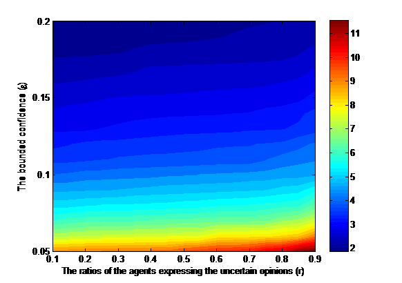
**Figure 1**. The average NC values under different r and $\varepsilon$ values.

Figure 1 shows two findings: (i) The average NC values increase as r increases, and (ii) the average NC values decrease as $\varepsilon$ increases. This implies that the larger ratios of the agents expressing the uncertain opinions will lead to more clusters. The opposite results will be obtained with the increase in the bounded confidences. These two observations from Figure 1 can be explained as follows: In the simulation, we find that with the increase in the ratios of the agents expressing the uncertain opinions and the decrease in the bounded confidences, the interactions among the agents will decrease. As a result, more clusters will appear.

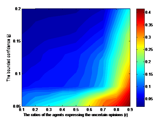
**Figure 2**. The average *r_ESC* values under different r and $\varepsilon$ values.

Figure 2 shows two findings: (i) The average r_ESC values increase as r increases, and (ii) The average r_ESC values decrease as $\varepsilon$ increases. This implies that the ratios of the extremely small clusters in all clusters will increase with the increase in the ratios of the agents expressing the uncertain opinions. The opposite result will be obtained with the increase in the bounded confidences. These two observations can be explained as follows: In the simulation, we find that the number of the isolated opinions at t = 0 will increase with the increase in the ratios of the agents expressing the uncertain opinions and the decrease in the bounded confidences. Consequently, the larger ratios of the extremely small clusters in all clusters will appear.

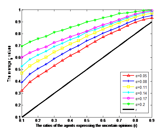
**Figure 3**. The average *r_s* values under different r and $\varepsilon$ values.

Figure 3 shows two findings: (i) The average r_s values increase as both r and $\varepsilon$ increase, and (ii) The average r_s values are larger than the r values. This implies that with the increase in the ratios of the agents expressing the uncertain opinions and the bounded confidences, the ratios of the agents expressing the uncertain opinions in the stabilized result will increase. Meanwhile, the ratios of the agents expressing the uncertain opinions in the stabilized result will be larger than those in the initial time. These two observations can be explained as follows: It is clear that the larger ratios of the agents expressing the uncertain opinions in the initial time will lead to the larger ratios of the agents expressing uncertain opinions in the stabilized result. Meanwhile, when interacting with the uncertain opinions, the exact opinions in the initial time will gradually become uncertain. Consequently, the larger ratios of the agents expressing the uncertain opinions in the stabilized result will be yielded.

The influences of the widths of uncertain opinions

We investigate the influences of the width of uncertain opinions based on three criteria NC, r_ESC and WU. In the simulation, let N = 500 and r = 1. We uniformly and randomly generate N exact numbers $y_i(0)$ $(i = 1,2, \ldots ,N)$ in [0, 1]. Based on the generated exact number, we randomly generate the uncertain opinions $\bar x_i (0) = [\bar x_i^L (0),\bar x_i^U (0)]$ $(i = 1,2, \ldots ,N)$, where $\overline{x}_i^L(0) = max \{ 0, y_i(0) - \delta_i \mathbin{/} 2 \}$ and $\overline{x}_i^U(0) = min \{ y_i(0)+ \delta_i \mathbin{/} 2, 1 \}$, and $\delta _i$ ($i = 1,2, \ldots ,N)$ is the exact number that is randomly selected from [0, $\lambda$]. Clearly, the widths of all of the generated uncertain opinions are smaller than $\lambda$. Furthermore, the larger $\lambda$ values indicate that all of the generated opinions are with the larger average widths. Next, using Eqs. (6) and (7) proceeds with the evolution of opinions. We set different $\lambda$ and $\varepsilon$ values and run each simulation 1000 times, obtaining the average NC , r_ESC and WU values under different parameters, which are shown in Figures 4-6.

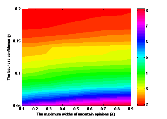
**Figure 4**. The average NC values under different $\lambda$ and $\varepsilon$ values.

Figure 4 shows the following finding: The average NC values increase as $\lambda$ increases. This implies that the number of clusters will increase with the increase in the widths of uncertain opinions.

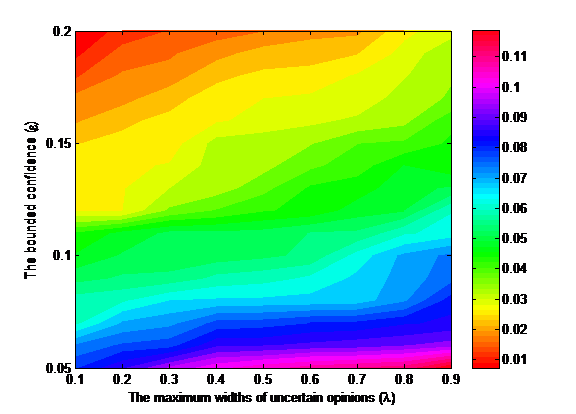
**Figure 5**. The average *r_ESC* values under different and $\varepsilon$ values.

Figure 5 shows the following finding: The average r_ESC values increase as $\lambda$ increases. This implies that the ratios of the extremely small clusters in all clusters will increase with the increase in the widths of uncertain opinions. The findings observed in Figure 4 and 5 can be explained as follows: In the simulation, we find that with the increase in the widths of uncertain opinions, the interactions among the agents will decrease, and the number of the isolated opinions will increase. As a result, more clusters and larger ratios of the extremely small clusters in all clusters will appear.

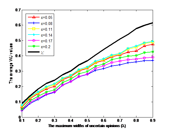
**Figure 6**. The average WU values under different $\lambda$ and $\varepsilon$ values.

Figure 6 shows the following findings: (i) The average WU values increase as $\lambda$ increases, and (ii) The average WU values are smaller than the $\lambda '$ values. This implies that the widths of uncertain opinions in the stabilized results will increase with the increase in the widths of uncertain opinions in the initial time. Meanwhile, the average widths of uncertain opinions in the stabilized result will be smaller than those in the initial time. It is clear that the larger widths of uncertain opinions in the initial time will lead to the larger widths of uncertain opinions in the stabilized result. Meanwhile, in the simulation, we find that the number of uncertain opinions with the smaller widths will increase in the dynamics of uncertain opinion formation. Consequently, the average widths of uncertain opinions in the stabilized result will become smaller.

The influences of the ratios of the agents with the uncertainty tolerances

We investigate the influences of the ratios of the agents with the uncertainty tolerances based on four criteria (i.e., NC, r_ESC, r_s andWU) mentioned in Section 4.1. Before investigating these influences, we denote the ratio of the agents with the uncertainty tolerances as $\beta$, where $\beta=\sharp A^u \mathbin{/} A$ and $\beta \in [0,1]$. Let the agent $A_i \in A^o$ and $A_j \in \tilde I(A_i ,\bar X(t))$. When confronting the uncertain opinion $[\bar x_j^L (t),\bar x_j^U (t)]$ ($\bar x_j^L (t) < \bar x_j^U (t)$), the agent $A_i$ will provide the accurate estimation $f_{ij} (t)$ as the opinion of $A_j$, where $f_{ij} (t) \in [\bar x_j^L (t),\bar x_j^U (t)]$. Notably, the accurate estimation $f_{ij} (t)$ in our simulation is randomly and uniformly selected from the uncertain opinion $[\bar x_j^L (t),\bar x_j^U (t)]$.

In the simulation, we randomly selected $N \times \beta$ agents from A, and assume that these selected $N \times \beta$ agents are with the uncertainty tolerances, i.e., the selected $N \times \beta$ agents belong to the set $A^u$ and the other agents belong to the set $A^o$. If the agent $A_i \in A^o$ and $A_j \in \tilde I(A_i ,\bar X(t))$, the agent $A_i$ will provide the accurate estimation $f_{ij} (t)$ as the opinion of $A_j$, where $f_{ij} (t)$ is randomly and uniformly generated from $[\bar x_j^L (t),\bar x_j^U (t)]$. Next, we use the methods in sections 4.3 and 4.4 to generate the initial opinions $\bar X(0)$, and use Eqs. (6)-(9) to calculate the $NC$, $r_{ESC}$, $r_s$ and $WU$ values. Finally, we set $\varepsilon = 0.1$ and different $\beta $, $r$ and $\lambda$ values, and run the simulation 1000 times, obtaining the average $NC$, $r_{ESC}$, $r_s$ and $WU$ values under different parameters, which are shown in Figures 7-9.

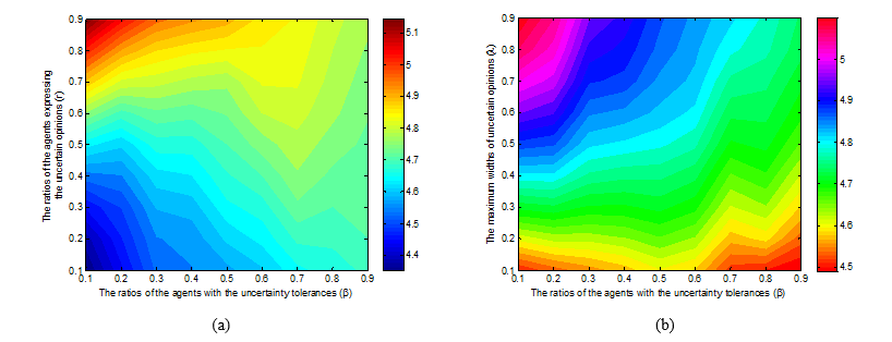
**Figure 7**. (a) The average NC values under different $\beta$ and r values; (b) The average NC values under different $\beta$ and $\lambda$ values.

Figures 7(a)-7(b) show the following findings: $r \ge 0.8$ or $\lambda\ge 0.5$, the average NC values decrease as $\beta$ increases. The finding implies that when the ratios of the agents expressing uncertain opinions or the widths of uncertain opinions are sufficiently large, the number of clusters will decrease with the increase in the ratios of the agents with the uncertainty tolerances. The findings in Figures 7(a)-7(b) can be explained as follows: In the simulation, when the ratios of the agent expressing uncertain opinions or the widths of uncertain opinions are sufficiently large, we find that the number of agents in the confidence sets will increase with the increase in the agents with the uncertainty tolerances. Consequently, less clusters will appear.

**Figure 8**. (a) The average *r_ESC* values under different $\beta$ and r values; (b) The average *r_ESC* values under different $\beta$ and $\lambda$ values.

Figures 8(a)-8(b) show the following finding: When $r \ge 0.7$ or $\lambda \ge 0.4$, the average r_ESC values decrease as $\beta$ increases. This implies that when the ratios of the agents expressing uncertain opinions or the widths of uncertain opinions are sufficiently large, the ratios of the extremely small clusters in all clusters will decrease with the increase in the ratios of the agents with the uncertainty tolerances. The findings in Figure 8(a)-8(b) can be explained as follows: In the simulation, when the ratios of the agents expressing uncertain opinions or the widths of uncertain opinions are sufficiently large, we find that the number of isolated opinions in the dynamics of uncertain opinion formation will decrease with the increase in the ratios of the agents with the uncertainty tolerances. Consequently, the smaller ratios of the extremely small clusters in all clusters will appear.

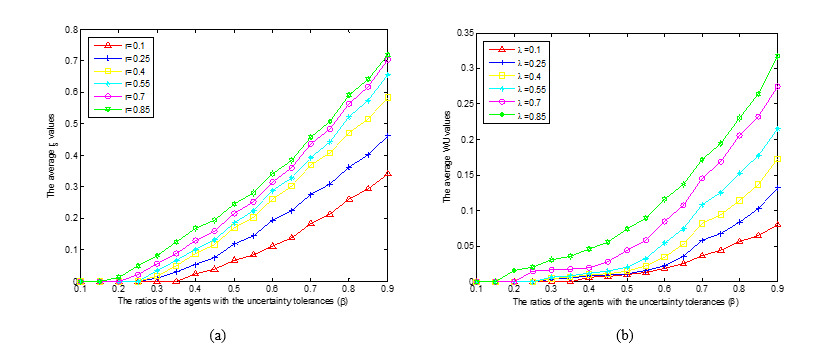
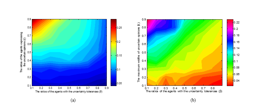
**Figure 9**. (a) The average *r_s* values under different $\beta$ and r values; (b) The average WU values under different $\beta$ and $\lambda$ values.

Figures 9(a)-9(b) show the following finding: The average r_s and WU values increase as $\beta$ increases. This implies that both the ratios of the agents expressing the uncertain opinions and the average widths of uncertain opinions in the stabilized results will increase with the increase in the ratios of the agents with the uncertainty tolerances. The findings in Figure 9(a)-9(b) can be explained as follows: In the simulation, we find that the opinions of the agents without the uncertainty tolerances will gradually become more accurate in the dynamics of uncertain opinion formation. Thus, with the increase in the ratios of the agents with the uncertainty tolerances, the larger ratios of the agents expressing uncertain opinions and the larger average widths of uncertain opinions in the stabilized result will appear.

Conclusions

In this study, we investigate the dynamics of uncertain opinion formation based on the bounded confidence model. In the proposed model, the agents express their opinions by using either numerical intervals (i.e., the uncertain opinions) or exact numbers (i.e., the exact opinions). Furthermore, based on different communication regimes, the agents are divided into two types: the agents with uncertainty tolerances and the agents without uncertainty tolerances.

We use an agent-based simulation to obtain the following findings: (i) With the increase in the ratios of the agents expressing uncertain opinions and the widths of uncertain opinions, more clusters and larger ratios of the extremely small clusters in all clusters will appear. Meanwhile, when the ratios of the agents expressing uncertain opinions or the widths of uncertain opinions are sufficiently large, less clusters and smaller ratios of the extremely small clusters in all clusters will appear with the increase in the ratios of the agents with the uncertainty tolerances; (ii) When all the agents are with the uncertainty tolerances, the ratios of the agents expressing the uncertain opinions in the stabilized result will be larger than those in the initial time. But the average widths of uncertain opinions in the stabilized result will be smaller than those in the initial time; (iii) When there exist certain agents without the uncertainty tolerances, both the ratios of the agents expressing the uncertain opinions and the average widths of uncertain opinions in the stabilized results will be smaller than those in the initial time.

The proposed model can be applied to address certain opinion formation problems in the real world. For example, when the government attempts to analyse the dynamics of public opinions on introducing a chemical project, certain citizens may express uncertain opinions on the necessity of introducing the chemical project. Furthermore, different citizens who encountered uncertain opinions have different uncertainty tolerances.

Generally, people express their opinions, sentiments, or support emotions regarding different issues in a social network. However, in this paper, the influences of different social network structures on uncertain opinion formation are not considered. Therefore, it would be an interesting future topic to investigate the dynamics of uncertain opinion formation by considering different social network structures.

Acknowledgements

Yucheng Dong would like to acknowledge the financial support of grants (Nos. 71171160, 71571124) from NSF of China, and grants (Nos. skqy201606 and skgt201502) from Sichuan University.

Appendix

Appendix A. Model analysis

In model analysis, we devote to compare the HK model with the proposed model and discuss some desired properties in the proposed model.

Firstly, in the comparative analysis, we show that the proposed model does not satisfy certain properties of the isolated fully connected group presented in the HK model. An isolated fully connected group (Urbig et al. 2008) is a set of agents in which all agents within the same group have a distance smaller than $\varepsilon$, whereas each agent outside the group has a distance larger than $\varepsilon$ to each agent in the group. Here, the distance measure in Eq. (3) is used to define the isolated fully connected group.

Generally, the HK model satisfies four properties as follows:

(i)An isolated fully connected group never splits;
(ii)The mean opinions of the agents in an isolated fully connected group remain stable;
(iii)Different isolated fully connected groups never merge.

In the following, we propose three counterexamples to illustrate that the proposed model does not satisfy (i)-(iii).

Example 1 is used to illustrate that (i) is not satisfied in the proposed model. In example 1, there are four agents $A_1 ,A_2 ,A_3 ,A_4 \in A^o$. Their initial opinions are given by

$$ x_i (0) = \left\{ {\begin{array}{*{20}c} {[0.19,0.3],} \hfill & {i = 1} \hfill \\ {[0.2,0.3],} \hfill & {i = 2} \hfill \\ {[0,0.1],} \hfill & {i = 3} \hfill \\ {[0.02,0.11],} \hfill & {i = 4} \hfill \\ \end{array}} \right.$$

(11)

,

We set the bounded confidence as: $\varepsilon=0.2$.

Based on Eq. (4), we find that $d(\bar x_i (t),\bar x_j (t)) \le \varepsilon$, for $i,j = 1,2,3,4$ and $i\neq j$. This indicates that the four agents have formed an isolated fully connected group. The initial accurate estimations of $A_1$, $A_2$, $A_3$ and $A_4$ are given as follows: $ A_1$: $f_{12} (0) = 0.3$, $f_{13} (0) = 0$, $f_{14} (0) = 0.02$; $A_2$: $f_{21} (0) = 0.3$, $f_{23} (0) = 0$, $f_{24} (0) = 0.02$; $A_3$: $f_{31} (0) = 0.3$, $f_{32} (0) = 0.3$, $f_{34} (0) = 0.02$; $A_4$: $f_{41} (0) = 0.3$, $f_{42} (0) = 0.3$, $f_{43} (0) = 0$.

Based on Eqs. (8)-(9), we obtain:

$$ x_i (1) = \left\{ {\begin{array}{*{20}c} {[0.245,0.3],} \hfill & {i = 1} \hfill \\ {[0.25,0.3],} \hfill & {i = 2} \hfill \\ {[0.01,0.06],} \hfill & {i = 3} \hfill \\ {[0.01,0.055],} \hfill & {i = 4} \hfill \\ \end{array}} \right.$$

(12)

We find: $d(\bar x_1 (1),\bar x_2 (1)) \le \varepsilon$, $d(\bar x_3 (1),\bar x_4 (1)) \le \varepsilon$ and $d(\bar x_l (1),\bar x_k (1))> \varepsilon$, for l = 1, 2 and k = 3, 4. Clearly, the agents A₁ and A₂ form an isolated fully connected group at time t = 1, and the agents A₃ and A₄ form the other isolated fully connected group at time t = 1.

Example 2 is used to illustrate that (ii) is not satisfied in the proposed model. In example 2, there are five agents, $A_1$, $A_2$, $A_3$, $A_4$ and $A_5$, where $A_1 ,A_3 ,A_5 \in A^u$ and $A_2 ,A_4 \in A^o $. Their initial opinions are given by

$$ x_i (0) = \left\{ {\begin{array}{*{20}c} {[0.1,0.3]} \hfill & {i = 1} \hfill \\ {0.05,} \hfill & {i = 2} \hfill \\ {0.25,} \hfill & {i = 3} \hfill \\ {[0,0.2],} \hfill & {i = 4} \hfill \\ {0.1,} \hfill & {i = 5} \hfill \\ \end{array}} \right.$$

(13)

We set the bounded confidence as: $\varepsilon=0.2$.

Based on Eq. (4), we find that $d(\bar x_i (0),\bar x_j (0)) \le \varepsilon$, for $i,j=1,2,\ldots,5$ and $i\neq j$. This statement indicates that the five agents have formed an isolated fully connected group. Additionally, the mean opinion (i.e., the average values for $\bar x_i (0)$) in this isolated fully connected group is equal to [0.10, 0.18].

The initial accurate estimations of agents A₂ and A₄ are given as follows: $A_2$: $f_{21} (0) = 0.25$, $f_{23} (0) = 0.25$, $f_{24} (0) = 0.1$, $f_{25} (0) = 0.1$; $A_4$: $f_{41} (0) = 0.2$, $f_{42} (0) = 0.05$, $f_{43} (0) = 0.25$, $f_{45} (0) = 0.1$.
Based on Eqs. (6)-(9), we obtain:

$$\bar x_i (1) = \left\{ {\begin{array}{*{20}c} {[0.10,0.18],} \hfill & {i = 1} \hfill \\ {0.15,} \hfill & {i = 2} \hfill \\ {[0.10,0.18],} \hfill & {i = 3} \hfill \\ {[0.12,0.16],} \hfill & {i = 4} \hfill \\ {[0.10,0.18],} \hfill & {i = 5} \hfill \\ \end{array}} \right.$$

(14)

We find that $d(\bar x_i (1),\bar x_j (1)) \le \varepsilon$, for $i,j=1,2,\ldots,5$ and $i\neq j$. This statement indicates that the five agents remain in an isolated fully connected group. However, the mean opinion at time t = 1 is equal to [0.114, 0.17].

Example 3 is used to illustrate that (iii) is not satisfied in the proposed model. In example 3, there are four agents $A_1, A_2, A_3$ and $A_4$, where $A_1, A_2, A_3 ,A_4 \in A^o$. The agents’ initial opinions are given by

$$\bar x_i (0) = \left\{ {\begin{array}{*{20}c} {[0.245,0.3],} \hfill & {i = 1} \hfill \\ {[0.25,0.3],} \hfill & {i = 2} \hfill \\ {[0.01,0.06],} \hfill & {i = 3} \hfill \\ {[0.01,0.055],} \hfill & {i = 4} \hfill \\ \end{array}} \right.$$

(15)

and the bounded confidence is assumed as: $\varepsilon=0.2$.

Based on Eq. (4), we find that two isolated fully connected groups exist that are formed at time t= 0. Specifically, agents A₁ and A₂ formed one isolated fully connected group, and agents A₃ and A₄ formed the other isolated fully connected group.

The initial accurate estimations of $A_1$, $A_2$, $A_3$ and $A_4$ are given as follows: $ A_1$: $f_{12} (0) = 0.25$; $A_2$: $f_{21} (0) = 0.245$; $A_3$: $f_{34} (0) = 0.055$; $A_4$: $f_{43} (0) = 0.06$.

Based on Eqs. (8)-(9), we obtain:

$$\bar x_i (1) = \left\{ {\begin{array}{*{20}c} {[0.2425,0.275],} \hfill & {i = 1} \hfill \\ {[0.2425,0.2725],} \hfill & {i = 2} \hfill \\ {[0.0325,0.0575],} \hfill & {i = 3} \hfill \\ {[0.035,0.0575],} \hfill & {i = 4} \hfill \\ \end{array}} \right.$$

(16)

Assume that: $f_{12} (t) = f_{21} (t) = 0.2425$, and $f_{34} (t) = f_{43} (t) = 0.0575$, for $t \ge 1$. Then, based on Eqs. (8) and (9), we obtain:

$$\bar x_i (t) = \left\{ {\begin{array}{*{20}c} {[0.2425,\frac{{0.275 + 0.2425(1 + 2 + \cdots 2^{t - 1} )}}{{2^t }}],} \hfill & {i = 1} \hfill \\ {[0.2425,\frac{{0.2725 + 0.2425(1 + 2 + \cdots 2^{t - 1} )}}{{2^t }}],} \hfill & {i = 2} \hfill \\ {[\frac{{0.0325 + 0.0575(1 + 2 + \cdots 2^{t - 1} )}}{{2^t }},0.0575],} \hfill & {i = 3} \hfill \\ {[\frac{{0.035 + 0.0575(1 + 2 + \cdots 2^{t - 1} )}}{{2^t }},0.0575],} \hfill & {i = 4} \hfill \\ \end{array}} \right.\,\,\,\,\,\,\,\,,t\geq 2.$$

(16)

Because $\mathop {\lim }\limits_{t \to \infty } \frac{{0.275 + 0.2425(1 + 2 + \cdots 2^{t - 1} )}}{{2^t }} = \frac{{0.275 + 0.2425(2^t - 1)}}{{2^t }} = 0.2425$, then we obtain: $\mathop {\lim }\limits_{t \to \infty } x_1 (t) = 0.2425$. Similarly, we have: $\mathop {\lim }\limits_{t \to \infty } x_2 (t) = 0.2425$ and $\mathop {\lim }\limits_{t \to \infty } x_3 (t) = \mathop {\lim }\limits_{t \to \infty } x_4 (t) = 0.0575$. Assume that $x_1 (t') = x_2 (t') = 0.2425$ and $x_3 (t') = x_4 (t') = 0.0575$, Because $\varepsilon=0.2$ and $d(\bar x_i (t'),\bar x_j (t'))\leq\varepsilon$, for $i,j = 1,2,3,4$ and $i\neq j$, then the four agents $A_1$, $A_2$, $A_3$ and $A_4$ formed an isolated fully connected group at time $t'$.

Then, two desired properties in the proposed model are discussed. The first property (see Property 1) indicates that the opinions of the agents without uncertainty tolerances will gradually become more accurate in the dynamics of uncertain opinion formation. The second property (see Property 2) indicates that all of the agents will hold an exact opinion when a consensus among the agents is achieved. The two desired properties are provided as follows:

Property 1. Let $\bar x_i (t) = [\bar x_i^L (t),\bar x_i^U (t)]$ be as defined previously, and let $d_i(t)$ be the width of the opinion $\bar x_i (t)$ , where $d_i (t) = \bar x_i^U (t) - \bar x_i^L (t)$. If agent $A_i \in A^o$, $d_i (t + 1) \le d_i (t)$, for $t = 0,1, \ldots$;

Proof. Without loss of generality, we assume that $A_i \in A^o$. Based on Eqs. (7)-(8), if A_i expresses the initial opinions using an exact number, A_i will continue expressing the exact opinions at any time. If A_i expresses the uncertain opinion $[\bar x_i^L (t),\bar x_i^U (t)]$ $(\bar x_i^U (t)>\bar x_i^L (t)$) at time t, $\bar x_i^U (t + 1) - \bar x_i^L (t + 1) = w_{ii} (t)\bar x_i^U (t) + \sum\limits_{A_j \in \tilde I(A_i ,\bar X(t)),j \ne i} {w_{ij} (t)f_{ij} (t)} - w_{ii} (t)\bar x_i^L (t) - \sum\limits_{A_j \in \tilde I(A_i ,\bar X(t)),j \ne i} {w_{ij} (t)f_{ij} (t)}$ = $w_{ii} (t)(\bar x_i^U (t) - \bar x_i^L (t))$

Because $0 \le w_{ii} (t) \le 1$, then $\bar x_i^U (t + 1) - \bar x_i^L (t + 1) \le \bar x_i^U (t) - \bar x_i^L (t)$. Clearly, $d_i (t + 1) \le d_i (t)$. This completes the proof.

Property 2 . Let $\bar x_i (t) = [\bar x_i^L (t),\bar x_i^U (t)]$ and $d_i (t)$ be as defined previously. Assume that a consensus among the agents is achieved at time t. Then, $d_i (t) = 0$, for $i = 1,2, \ldots ,N$.

Proof. Let $[\bar x_c^L ,\bar x_c^U ]$ be the uniform opinion of all of the agents at time t . Let $A_i$ and $A_j$ be any two agents, where $A_i\in A^o$ and $A_j\in A^u$. Based on Eqs. (6)-(9), we obtain: $\bar x_i^L (t + 1) = \frac{1}{N}\bar x_c^L + \sum\limits_{A_j \in \tilde I(A_i ,\bar X(t)),j \ne i} {\frac{{f_{ij} (t)}}{N}}$, $\bar x_i^U (t + 1) = \frac{1}{N}\bar x_c^U + \sum\limits_{A_j \in \tilde I(A_i ,\bar X(t)),j \ne i} {\frac{{f_{ij} (t)}}{N}}$. and $\bar x_j^L (t + 1) = \frac{1}{N}\bar x_c^L + \sum\limits_{A_j \in \tilde I(A_i ,\bar X(t)),j \ne i} {\frac{{\bar x_c^L }}{N}} = \bar x_c^L$, $\bar x_j^U (t + 1) = \frac{1}{N}\bar x_c^U + \sum\limits_{A_j \in \tilde I(A_i ,\bar X(t)),j \ne i} {\frac{{\bar x_c^U }}{N}} = \bar x_c^U$.
Because the consensus among all of the agents remains stable, then: $\bar x_i^L (t + 1) = \bar x_j^L (t + 1) = \bar x_c^L$ and $\bar x_i^U (t + 1) = \bar x_j^U (t + 1) = \bar x_c^U$. Furthermore, we have: $\frac{{f_{ij} (t)}}{N} = \frac{{\bar x_c^L }}{N} = \frac{{\bar x_c^U }}{N}$. As a result, $f_{ij} (t) = \bar x_c^L = \bar x_c^U$.

This completes the proof.

References

AFSHAR, M. & Asadpour M. (2010). Opinion formation by informed agents. Journal of Artificial Societies and Social Simulation, 13(4) 5: https://www.jasss.org/13/4/5.html. [doi:10.18564/jasss.1665]

BLONDEL, V.D., Hendrickx, J.M. & Tsitsiklis, J.N. (2009). On Krause's multi-agent consensus model with state-dependent connectivity. IEEE Transactions on Automatic Control, 54(11), 2586-2597. [doi:10.1109/TAC.2009.2031211]

CERAGIOLI, F. & Frasca, P. (2012). Continuous and discontinuous opinion dynamics with bounded confidence. Nonlinear Analysis: Real World Applications, 13(3), 1239–1251 [doi:10.1016/j.nonrwa.2011.10.002]

DEFFUANT, G., Carletti, T. & Huet, S. (2013). The Leviathan model: Absolute dominance, Generalised distrust, small worlds and other patterns emerging from combining vanity with opinion propagation. Journal of Artificial Societies and Social Simulation, 16 (1) 5:https://www.jasss.org/16/1/5.html. [doi:10.18564/jasss.2070]

DEFFUANT, G., Neau D., Amblard F. & Weisbuch G. (2000). Mixing beliefs among interacting agents. Advances in Complex Systems 3(01n04) 87-98. [doi:10.1142/S0219525900000078]

DE GROOT M.H. (1974). Reaching a consensus. Journal of American Statistic Association, 69, 118-121. [doi:10.1080/01621459.1974.10480137]

DONG, Y.C., Zhang, G.Q., Hong, W.C. & Yu, S. (2013). Linguistic computational model based on 2-tuples and intervals. IEEE Transactions on Fuzzy Systems, 21(6), 1006-1018. [doi:10.1109/TFUZZ.2013.2239650]

DONG, Y.C., & Herrera-Viedma, E. (2015). Consistency-driven automatic methodology to set interval numerical scales of 2-tuple linguistic term sets and its use in the linguistic GDM with preference relation. IEEE Transactions on Cybernetics, 45(4), 780-792. [doi:10.1109/TCYB.2014.2336808]

ETESAMI, S.R, Basar, T., Nedic, A. & Touri, B. (2013). Termination time of multidimensional Hegselmann -Krause opinion dynamics. Proceedings of the American Control Conference, 1255 - 1260. [doi:10.1109/acc.2013.6580008]

FORTUNATO, S, Latora, V, Pluchino, A. & Rapisarda, A. (2005). Vector opinion dynamics in a bounded confidence consensus model. International Journal of Modern Physics C, 16(10): 1535-1551. [doi:10.1142/S0129183105008126]

FRENCH, J.R.P. (1956). A formal theory of social power. Psychological Review, 63, 181-194. [doi:10.1037/h0046123]

FRIEDKIN, N.E. & Johnson, E.C. (1990). Social influence and opinions. Journal of Mathematical Society, 15, 193-206. [doi:10.1080/0022250X.1990.9990069]

HEGSELMANN, R., König, S., Kurz, S., Niemann, C. & Rambau, J. (2015). Optimal opinion control: The campaign problem. Journal of Artificial Societies and Social Simulation, 18(3) 18: https://www.jasss.org/18/3/18.html. [doi:10.18564/jasss.2847]

HEGSELMANN, R. & Krause, U. (2002). Opinion dynamics and bounded confidence models, analysis, and simulation. Journal of Artificial Societies and Social Simulation, 5(3) 2 : https://www.jasss.org/5/3/2.html.

KRAPIVSKY, P. & Redner, S. (2003). Dynamics of majority rule in two-state interacting spin systems. Physical Review Letters, 90(23). [doi:10.1103/PhysRevLett.90.238701]

LORENZ, J. (2005). A stabilization theorem for dynamics of continuous opinions, Physica A: Statistical Mechanics and its Applications, 355(1), 217-223.

LAGUNA, M.F., Abramson, G. & Zanette, D.H. (2003). Vector opinion dynamics in a model for social influence. Physica A: Statistical Mechanics & Its Applications, 329: 459-472. [doi:10.1016/S0378-4371(03)00628-9]

LATANE, B. (1981). The psychology of social impact. American Psychologist, 36(4), 343-356. [doi:10.1037/0003-066X.36.4.343]

LIM, D.W., Lee, H.S., Zo, H.J. & Ciganek, A. (2014). Opinion formation in the digital divide. Journal of Artificial Societies and Social Simulation, 17 (1) 13 :https://www.jasss.org/17/1/13.html. [doi:10.18564/jasss.2366]

MCKEOWN, G. & Sheehy, N. (2006). Mass media and polarisation processes in the bounded confidence model of opinion dynamics. Journal of Artificial Societies and Social Simulation, 9 (1) 11 : https://www.jasss.org/9/1/11.html.

MORARESCU, I.-C. & Girard, A. (2011). Opinion dynamics with decaying confidence: Application to community detection in graphs. IEEE Transactions on Automatic Control, 56(8), 1862–1873 [doi:10.1109/TAC.2010.2095315]

PINEDA, M., Toral, R. & Hernández-García, E. (2009). Noisy continuous-opinion dynamics. Journal of Statistical Mechanics Theory & Experiment, 32(1): 55-62. [doi:10.1088/1742-5468/2009/08/p08001]

PINEDA, M. & Toral, R. & Hernández-García, E. (2013). The noisy Hegselmann-Krause model for opinion dynamics. The European Physical Journal B, 86, 490-499. [doi:10.1140/epjb/e2013-40777-7]

RIGHI S. & Carletti T. (2009). The influence of social network topology in an opinion dynamics model. Proceeding of the European Conference on Complex Systems.

SALZARULO, L. (2006). A continuous opinion dynamics model based on the principle of meta-contrast. Journal of Artificial Societies and Social Simulation, 9 (1) 13 : https://www.jasss.org/9/1/13.html.

SUTTON, J.L., Cosenzo, K.A. & Pierce, L.G. (2004). Influence of culture & personality on determinants of cognitive processes under conditions of uncertainty. Army Research Lab Fort Sill Ok Human Research And Engineering Dir.

URBIG, D., Lorenz, J. & Herzberg, H. (2008). Opinion dynamics: The effect of the number of peers met at once. Journal of Artificial Societies and Social Simulation, 11(2) 4:https://www.jasss.org/11/2/4.html.

WANG, H.J. & Shang, L.H. (2015). Opinion dynamics in networks with common-neighbors-based connections. Physica A, 421, 180-186. [doi:10.1016/j.physa.2014.10.090]

WEISBUCH, G. (2004). Bounded confidence and social networks. The European Physical Journal B-Condensed Matter and Complex Systems, 38(2), 339-343. [doi:10.1140/epjb/e2004-00126-9]