
Introduction
The effects of innovation on employment are still a controversial issue in economic thought (Vivarelli 2014). Indeed, while some authors defend the fact that advances in technology will ultimately have a positive impact on the general level of employment of a given economy, the problem of “technological unemployment” is still a concern for many economists (Vivarelli 2014).
This issue has a distinct relevance nowadays, as we are seeing tremendous technological developments, particularly in the field of Artificial Intelligence (AI), which threaten to render obsolete the involvement of humans in numerous tasks (Ford 2015). As a result, automation and its remarkable potential for the disruption, not only of the manufacturing sector (a trend known as “Industry 4.0”), but also of the services sector, has become an issue of major priority for business leaders around the globe (Manyika et al. 2017). Nonetheless, automation is not simply a concern for the corporate sphere, but rather a phenomenon with potentially massive economic and social implications. Indeed, as pointed out by DeCanio in a recent study which examines the potential effects of the spread of Artificial Intelligence technologies on wages, it has been estimated that 40%-50% of the workforce is vulnerable to being replaced by AI in the next couple of decades (DeCanio 2016). However, DeCanio begins his analysis by recognizing it is currently widely accepted that technological change can increase employment in some occupations or sectors, while decreasing it in others (DeCanio 2016), which means there remain questions to be answered regarding the overall effect of innovation on employment.
Given the complexity of these issues, and the inability of both theoretical and empirical approaches to provide a clear answer to the questions at hand, an agent-based approach presents itself as a promising alternative for attempting to answer this puzzle. Agent-based models have been commonly used within the evolutionary economics perspective, which provides much more realistic settings than neoclassical economics by allowing the consideration of learning agents acting in a context of disequilibrium and bounded-rationality (Silva 2009). Furthermore, the possibilities inherent to agent-based systems are particularly useful for understanding innovation processes, and these models have already been successfully used in explaining empirical stylized facts regarding innovation (Dawid 2006).
Bearing this in mind, this paper presents an agent-based model developed in Python, using the Mesa framework, with the purpose of allowing a qualitative study of the controversial relationship between innovation and employment. It is not the ambition of this model to accurately mimic past quantitative empirical data or predict future levels of employment.
This paper is structured as follows. After this overview, Section 2 presents a brief survey of the main theoretical and empirical approaches on the effects of innovation on employment. On Section 3, a literature review is presented regarding agent-based modelling, both from the perspective of economic applications and from a methodological perspective. Following, Section 4 presents the main features of the model developed. Section 5 contains the results of the simulations performed on the model, as well as a series of analysis of those results. Finally, Section 6 presents the Concluding Remarks of this paper, including mentions to limitations of this work and potential future research paths.
Main perspectives on the Innovation and Employment Nexus
It is important to start by distinguishing between process innovation, which may allow for the production of the same amount of output with a lower amount of labour, and product innovation, which allows for the introduction of new products into the market. As it is straightforward to conclude, process innovation has a direct labour-saving effect, thus having a direct negative influence on employment. The effects of product innovation will be addressed later in this literature review.
Besides the direct labour-saving effect of process innovation, economic theory has proposed an indirect way through which innovation may have a negative effect on employment: the creative destruction effect. Introduced by Schumpeter (1943), the concept of creative destruction was first used as a mechanism in a dynamic model of growth for studying unemployment by Aghion & Howitt (1994). Since then, the creative destruction effect has become one of the most widely used mechanisms in economic literature for understanding the relationship between innovation, growth and unemployment (Neto & Silva 2013).
In a recent survey, Vivarelli presents a comprehensive and systematic review of the economic literature on the relationship between innovation and employment, both from a theoretical and empirical perspective (Vivarelli 2014). The author begins his analysis by enumerating a series of mechanisms, identified by economists, which can counterbalance the initial labour-saving effect of innovation, consisting of what Karl Marx named the “compensation theory”. Having enumerated the compensation mechanisms proposed by the economic theory, Vivarelli further identifies the criticisms and limitations identified for these mechanisms, concluding that they do not provide a conclusive answer regarding the impact of innovation on employment. Regarding empirical studies on the relationship between innovation and employment, Vivarelli further concludes that this approach does not allow for a definite conclusion on this matter either, since empirical studies have their own limitations and they do not seem to yield consensual results (Vivarelli 2014).
More recently, Stare & Damijan (2015) focused on the consequences, for employment and skills, of the innovation spillovers from vertically linked sectors. This study allows for the conclusions that spillovers of product innovations have a significant positive effect on employment and skill upgrading for the firms benefiting from those spillovers, whereas spillovers of process innovation in vertically linked sectors have a negative effect on employment growth and skill composition for firms subject to those spillovers.
Within the empirical literature on this issue, the topic of AI has deserved growing attention lately. Indeed, in a recent study, DeCanio investigates the effects of the spread of AI on wages, concluding that for a level of elasticity of substitution between human and robotic labour greater than the 1.7–2.1 range, the spread of AI technologies will lead to a decrease in aggregate wages (DeCanio 2016).
Main perspectives on agent based modelling
As Axelrod & Tesfatsion put it, agent-based modelling (ABM) is a method for studying systems composed of interacting agents and exhibiting emergent properties, that is, exhibiting properties arising from the interactions of the agents that cannot be deduced from the properties of the agents themselves (Axelrod & Tesfatsion 2005). Furthermore, multi-agent models are particularly appealing for their ability to study the interactions of heterogeneous agents, characterized by learning and bounded rationality (Safarzyńska & van den Bergh 2010).
ABM of economic phenomena, also known as Agent-based Computational Economics (ACE), has received growing attention in recent years due, to a great extent, to the inadequacy demonstrated by the prevailing theoretical frameworks for economic analysis, during and after the global financial crisis of 2007-2008. In this context, ACE has been proposed as a relevant and promising alternative framework for economic analysis (Bouchaud 2008; Fagiolo & Roventini 2017; Farmer & Foley 2009). Furthermore, ACE models have been extensively used as a “laboratory” for policy design, in addition to being widely successful in explaining micro and macro stylized facts (Fagiolo & Roventini 2017).
Regarding Agent-Based Models (ABMs) considering either innovation or labour market dynamics separately, these are quite common in Agent-based Computational Economics (ACE). However, when it comes to combining both dynamics (innovation and labour market), the literature is surprisingly scarce. Nonetheless, two studies combining both sides of the equation stand out. In their paper, Fagiolo et al. (2004) present an ABM of output and labour-market dynamics in which labour productivities change due to technical progress. However, the model portrays technical change in a simplistic way, without considering the firms’ decisions regarding innovation (Dawid 2006). In a more recent study, Silva et al. (2012) take a similar approach to Fagiolo et al. (2004), but considering two types of workers, routine and non-routine, as well as firms with heterogeneous institutional settings. Despite being more realistic and complex than Fagiolo’s approach, this model still represents technological change in a rather simple way.
Finally, and despite recent methodological advances, agent-based modelling is still subject to methodological concerns, in particular the definition of an adequate and generally accepted protocol for describing an ABM in a transparent manner (Tesfatsion 2016). It should be noted that some attempts have already been performed in this direction, such as: the “Overview, Design Concepts, Details” (ODD) Protocol for the description of ABMs (Grimm et al. 2010, 2013; Grimm & Railsback 2012); or the TRACE (TRAnsparent and Comprehensive Ecological modelling documentation) Protocol for documenting the steps to design, evaluate, and validate ABMs (Grimm et al. 2014); or even the Open Agent-Based Modelling Consortium, which attempted to create a community framework for agent-based modelling (Janssen et al. 2008).
Having presented, in this section, a literary review on ABM of economic phenomena and ABM methodological practices, the following section contains a description of the developed model.
The model
In this chapter, the developed ABM is presented. Regarding the implementation methodology, it is important to mention that the present ABM was developed in Python, using the Mesa framework (Masad & Kazil 2015). Mesa is an open-source Python package developed with the goal of becoming a Python-based alternative to popular ABM frameworks such as NetLogo, Repast, or MASON. In the following pages, we present the purpose of the model, its entities, its underlying principles and its mechanisms. For the model’s detailed programming code, please refer to Appendix B.
Purpose
The purpose of this model is to allow a qualitative study of the dynamics underlying the relationship between innovation and employment. It is not the ambition of this model to provide a set of quantitative outputs which accurately mimic past quantitative empirical data, nor to allow for a prediction of the future levels of employment in our societies. Rather, this model aims for three main goals.
First, the model intends to allow for a Gedankenexperiment (a thought experiment which is, generally, impossible to perform in the real world) on this issue, by providing the reader with a set of questions, hypothesis, and conclusions regarding the issue under analysis. Second, the model intends to present a representation of the reality in what concerns the relationship between innovation and employment, which is simultaneously: new in the economic literature, detailed enough to be more accurate than existing representations, and abstract enough to allow for valid general conclusions. Finally, the last goal of this ABM is to lay the groundwork for the development of more complex models revolving around its central concepts and dynamics.
Entities, state variables and scales
The model is composed by three main entities: tasks, firms (agents), and the economy (environment).
Tasks
The basic unit of the model is a task. In order to develop a certain amount of their product, firms need to complete a certain set of complementary tasks. Tasks are characterized by whether or not they are “automatable”, their “added value”, and the “activity” category they belong to.
Tasks than can be performed only by human labour are considered non-automatable, whereas tasks that can potentially be performed by either human labour or robotic labour are considered automatable. However, it should be noted that a firm can only perform a task using robotic labour if the firm has learnt how to automate that task.
The added value of a task reflects the contribution of that task to the overall value of an output unit. More specifically, the value of one unit of output, produced by a given firm, equals the average of the added value of the tasks performed by that same firm.
Tasks can belong to different activity categories. Some activities have a higher automation potential than others, that is, they include a higher proportion of automatable tasks than others. Regarding added value, there is no differentiation between activities, that is, the mechanism that generates the tasks in the model uses the same probability distribution, for the added value of tasks, across the different activity categories.
Firms (agents)
The agents in the model are firms. These agents produce output by performing tasks using human labour and robotic labour as inputs. In their attempt to maximize profits, firms will carry out technological change, in the form of process and product innovation. In this context, process innovation means automating a certain task in order to replace wage costs with capital costs (assumed to be lower), whereas product innovation means discovering a new task which allows the company to produce higher-value output, but which must be performed by humans (at least until it becomes automated). At each time step, firms are faced with the decision of performing either product or process innovation. The decision process which leads firms to choose between product or process innovation is described in gradually more detail in the following sections.
Table 1 summarizes the main attributes of a firm.
| Production | Budgeting |
| Known tasks: each firm has its own set of tasks which it knows how to perform Current tasks: a firm must decide on the 10 tasks it will perform at each time step Employees: the number of human labour units the firm employs at a given time step Robots: the number of robotic labour units the firm owns at a given time step Output quantity: the amount of output units the firm has produced at a given time step Unitary value of output: the value of each output unit the firm has produced at a given time step | Revenues: the product of a firm’s Output quantity and its Unitary value of output Salary costs: the product of a firm’s number of Employees and the Salary in the economy Robot costs: the costs a firm bears for owning robots (opportunity cost of the investment and depreciation costs) R&D stock: determines the likelihood that a firm’s innovation attempts will be successful R&D expenses: the fraction of a firm’s earnings that it will invest in R&D Operating net income: a firm’s revenues minus its operating costs |
Economy (environment)
In this model, the environment in which the agents (firms) interact is an economy containing attributes which, on the one hand influence their decisions, and on the other hand are affected by their decisions.
Table 2 summarizes the main attributes of an economy.
| Innovation | Labor market |
| R&D Intensity: determines the % of earnings that each firm will invest in R&D (equal for every firm, constant over time) Threshold Unitary Value of Output: a certain percentile of the observations of Unitary Value of Output for all firms in the economy, at a given time step. Firms will perform Product Innovation if their Unitary Value of Output is lower than the Threshold, and will perform Process Innovation if it is equal or higher. Product Innovation Propensity: the percentile rank used to compute the Threshold (ranging from 0 to 100). Therefore, in a simplistic manner, in an economy with a Product Innovation Propensity of X, at any given time step, X% of the firms will be performing Product Innovation, while the remaining ones will perform Process Innovation. | Active population: the fraction of the population that is either employed or actively seeking employment Employed population: the total number of employees in every firm in the model at a given time step Employment Rate: the fraction of the Active population which is Employed at a given time step Human share of input: the fraction of the total tasks performed, at a given time step, which are performed by humans Salary: since the model assumes that every employee has the same characteristics, it also assumes that they all receive the same salary Wage Share: the fraction of the total Output in the economy that has been distributed as Salaries, at a given time step |
Process overview and schedule
During a time step in a simulation, the following procedures take place:
- Firms’ actions: each of the firms in the model is activated in a random order and it performs its own schedule of procedures at the micro-level.
- Market dynamics: this procedure takes place at the macro-level and consists of a set of computations regarding the goods and services market and the labour market in the simulated economy.
- Reporting of output data: at this stage, the model stores data regarding the status of the economy and of its agents, namely innovation and labour market statistics.
- Replacement of bankrupt firms: before the period ends, the model replaces bankrupt firms with new firms incorporating characteristics which match the average of the characteristics of the surviving firms.
When a firm is activated, it performs the following actions:
- Choose the tasks to perform: out of all the tasks a firm knows how to perform, it needs to choose which tasks to perform at a given time step.
- Hire employees and acquire robots: having decided on which tasks to perform at a given time step, a firm must obtain the production inputs required to perform those tasks.
- Produce output: the execution of a firm’s chosen tasks by the obtained inputs results in a certain quantity of output with a certain unitary value.
- Budget: towards the end of its schedule, the firm must compute its revenues, costs, earnings, R&D budget, and its next period’s production expectations.
- Innovate: before its action ends, a firm must decide whether it wants to attempt product or process innovation, and observe the resulting outcome.
Basic principles
The model is governed by a series of underlying principles and simplifying assumptions regarding:
Product Innovation
Motivation for product innovation – by performing product innovation, firms increase their Unitary Output Value. As such, there are two motivations behind product innovation. The first is the fact that, by increasing its Unitary Output Value, for the same quantity of output, a firm increases its revenues and, therefore, its profits. The second is the firms’ belief that, by improving the quality of their product, they will increase their chances of winning market-share moving forward.
Decision criteria for product innovation – a firm will choose product over process innovation if its Unitary Value of Output is lower than the economy’s Threshold. The rationale behind this decision is as follows: a firm considers its position in the market to be threatened if the quality of its offering, compared to its competitors, falls below a certain threshold, and so its strategic focus becomes improving its products or services, rather than optimizing its processes.
Newly discovered tasks are manual at first – In the model, whenever a firm successfully performs product innovation and, as a result, a new task is added to its set of known tasks, that task is always initially manual. If the task in question is automatable, a firm can later learn how to perform it using robots (by means of process innovation), but, initially, it must always be performed by a human.
Product innovation is only incremental – the model considers that product innovation is merely the introduction of tasks in the productive process which allow for the creation of higher-value products. That is, the model doesn’t consider the possibility of disruptive product innovations that introduce entirely new products.
Process Innovation
Motivation for process innovation – The firms in the model perform process innovation with the goal of decreasing their costs. In fact, by being able to replace humans with robots in the performance of a given task, a firm is able to replace salary costs with the costs of owning and operating the robots, which are assumed to be lower.
Decision criteria for process innovation – a firm will choose process over product innovation if its Unitary Value of Output is equal to or higher than the economy’s Threshold. The rationale behind this decision is as follows: a firm considers its position in the market to be secure if the quality of its offering, compared to its competitors, is above a certain threshold, and so its strategic focus becomes optimizing its processes, rather than improving its products or services.
Automation potential – The automation potential of tasks belonging to each activity category was defined according to a McKinsey Global Institute report regarding the automation potential for activities in the US economy (Manyika et al. 2017). It should be noted that the definition of “automation potential” used in the report considers only the potential for automation resulting from the adaptation of currently demonstrated technologies. As such, while, in the real world, the automation potential of tasks may increase over time, in the model it was deemed stable, in order to keep the model simple and grounded in empiric research.
Cloud robotics – a firm’s knowledge regarding the automation of tasks is automatically and immediately shared with all the robot units it owns. This mechanism attempts to simulate the concept of cloud robotics, according to which robots are able to share the same knowledge and computational power by accessing a central storage and processing unit (Ford 2015).
Production
Full complementarity of the selected tasks – as previously mentioned, at each time step, each firm must select the 10 tasks it will perform. All of these 10 tasks need to be performed once in order to produce 1 unit of output, that is, they are complementary.
Full substitutability of the known tasks – Even though the 10 selected tasks are considered to be fully complementary once selected, a firm’s known tasks are considered to be fully substitutable during the selection process. That is, firms are allowed to select whichever 10 tasks they want from their set of Known Tasks, without replacement, and without any combination restriction.
Preference for value over profitability – the criteria used by firms to select the 10 tasks to be performed is their added-value, that is, their ability to add value to the firm’s output. The reasoning behind these criteria is rooted in the firms’ belief that, by providing their customers with a highly valuable product, they will be able to win, or not lose, market-share moving forward.
Unitary task-productivity of labour units – each unit of labour in the model, be it human or robotic, can perform only one task at each time step, and it can perform that task only once during that time step.
Preference for robots over humans in automated tasks – it is assumed that, whenever a task becomes automated, firms will always prefer to perform that task by using robots instead of humans. This assumption is rooted in two other assumptions of the model. The first is that it is possible for a robot to perform that task with the exact same quality standards as a human or with even higher quality standards. The second assumption is that it is always more costly to perform it using human labour than robotic labour.
Output market
One-period full market clearing – it is assumed in this model that every unit being produced is consumed in the same time step, that is, aggregate production necessarily creates an equal quantity of aggregate demand in the same period.
Intrinsic product value – the value of products in the model is assumed to be intrinsic to the products themselves, being a direct result of the tasks which were performed in order to produce it. As such, the value of the products is not considered to be subjective and does not reflect each consumer’s preferences. In a similar fashion, the price of a product is assumed to exactly match its value, meaning that there’s no consideration for inflation and prices are not considered to be, in any degree, a monetary phenomenon.
Constant and equal quantity market shares – firms’ market shares, measured in Output Quantities are considered to be equal for every firm at every time step. Nevertheless, it should be noted that firms are considered unable to perceive this model feature and, as previously mentioned, hold the belief that it is possible for them to win or lose customers. In fact, this belief ultimately determines firms’ innovation decisions, in such a way that it can be seen as an automatic stabilizer of quantity market-shares:
- Firms believe they are subject to competition via product differentiation, thus motivating them to perform product innovation if they are lagging behind the market, which in turn makes the intrinsic value of goods converge in the long run
- Firms believe they are subject to competition via price, thus motivating them to perform process innovation to reduce costs, which, under the assumption of homogeneous pricing strategies, makes the price of goods converge in the long run
As such, the fact that market shares remain stable can be interpreted as a consequence of convergent prices and intrinsic values in the long run, which can in turn be seen as the result of decisions firms take while being unaware of this simplifying assumption.
Employees / labour market
Active population – In this model, it is assumed that all the population is active. Additionally, the Active Population matches, at every time step, the total number of tasks that need to be performed in order to produce the Total Output Units in the economy, regardless of those tasks being performed by humans or robots. Therefore, the Active Population always grows at the same rate as the Total Output Units, which is a rate defined exogenously.
Homogeneity of human skills – workers are assumed to have the exact same skills, that is, they are assumed to be able to perform every task with the same quality standards.
No barriers to hiring or firing – firms in the model are able to hire and fire employees with total freedom, that is, at every time step, they can hire or fire as many employees as they which, without incurring any costs, and with immediate effect.
Inelastic labour demand – the demand for labour in the model does not depend on the Salary in the economy. In fact, the only factors affecting firms’ demand for labour units are their technology, that is, how many of their current tasks are manual or automated, and their planned production.
Linear labour supply – the supply of labour in the model is assumed to be linear, with 0 workers willing to be employed at a salary of 0, and all of the active population willing to be employed at a salary rate which matches the Average Expected Employee Productivity. As a consequence, the Salary in the economy will always match the product of the Employment Rate and the Average Expected Employee Productivity. An alternative way to interpret this relationship is by considering that the Employment Rate determines the bargaining power of employees, which in turn determines the portion of the Average Expected Employee Productivity that employees are able to capture in the form of salaries.
Sub-models
Agent actions
As previously mentioned, at each time step, firms must perform the following procedures:
- Choose the tasks to perform;
- Hire employees and acquire robots;
- Produce output;
- Budget;
- Innovate.
Choose the tasks to perform
Out of all the tasks a firm knows how to perform, it needs to choose 10 tasks to perform at a given time step. As mentioned before, the firm attempts to maximize the unitary value of its output at every step, so the tasks selected must be the ones with the highest added-value. In order to achieve this result, each firm follows these steps:
- Sort the set of known tasks by added-value;
- Select the top 10 tasks as current tasks.
Hire employees and acquire robots
Having decided on which tasks to perform at a given time step, a firm must obtain the production inputs required to perform those tasks, by following these steps:
- From the set of current tasks, identify the tasks that the firm has learned how to automate and the tasks that are manual;
- Count the number of automated and manual tasks, that is, the number of tasks that will be performed by robots and the number of tasks that will be performed by humans;
- Compute the number of employees and robots required by firm \(i\) during the time step \(j\):
$$\textit{Employees}_{i,j} = \textit{Round}(\textit{Expected Output}_{i,j} \ast \textit{Number of current manual tasks}_{i,j})$$ (1) $$\textit{Robots}_{i,j} = \textit{Round}(\textit{Expected Output}_{i,j} \ast \textit{Number of current automated tasks}_{i,j})$$ (2) - Hire the required production inputs (as mentioned before, the salary is defined at the macro-level, and it is assumed that the firm is able to obtain all the employees and robots it requires immediately).
Produce output
The execution of a firm’s chosen tasks by the obtained inputs results in a certain quantity of output with a certain unitary value. In order to compute these values, a firm must perform the following computations:
- The quantity of output units produced by a firm i at the time step j is given by:
$$\textit{Quantity of Output}_{i,j} = \min(\textit{Obtainable Output from Manual Tasks}_{i,j},\\ \textit{Obtainable Output from Automated Tasks}_{i,j})$$ (3) - This expression derives from the fact that all tasks are complementary: since manual and automated tasks are all complementary with each other (and not only within each group of tasks), the obtainable output from the firm as a whole is the minimum of what could be obtained if we considered each group of tasks separately. Moreover, the output that could be obtained considering each group of tasks separately equals the number of times the company can perform the whole set of tasks in that group, as detailed below.
- The Obtainable Output from Manual Tasks, i.e. the number of times the company can perform all the manual task, is computed through the integer division of the number of employees by the number of current manual tasks. If there are no manual tasks in the current tasks set, then the obtainable output from manual tasks is considered to be infinite, since it does not constitute a production bottleneck (that is, the Quantity of Output is not at all limited by the need to perform manual tasks).
- Similarly, the Obtainable Output from Automated Tasks, i.e. the number of times the company can perform all the automated task, is computed through the integer division of the number of robots by the number of current automated tasks. If there are no automated tasks in the current tasks set, then the obtainable output from automated tasks is considered to be infinite, since it does not constitute a production bottleneck (that is, the Quantity of Output is not at all limited by the need to perform automated tasks).
- The value of an output unit of firm i at the time step j is given by:
$$\textit{Unitary Value of Output}_{i,j} = \textit{Average}\Bigl(\textit{Current Task Set}_{i,j [\textit{Added-value}]}\Bigr)$$ (4)
Budget:
Towards the end of its schedule in step \(j\), a firm \(i\) computes its revenues, costs, earnings, R&D budget, and its production expectations for step \(j+1\):
| $$\textit{Revenues}_{i,j} = \textit{Quantity of Output}_{i,j} \ast \textit{Unitary Value of Output}_{i,j}$$ | (5) |
| $$\textit{Salary Costs}_{i,j} = \textit{Employees}_{i,j} \ast \textit{Salary in the Economy}_j$$ | (6) |
| $$\textit{Robot Costs}_{i,j} = \textit{Robots}_{i,j} \ast (\textit{Interest Rate} + \textit{Depreciation Rate})$$ | (7) |
| $$\textit{RD Expenses}_{i,j} = \begin{cases} 0\text{,} \text{if} \,\, \bigl( \textit{Revenues}_{i,j} - \textit{Salary Costs}_{i,j} - \textit{Robot Costs}_{i,j} \bigr) \leq 0\\ \bigl( \textit{Revenues}_{i,j} - \textit{Salary Costs}_{i,j} - \textit{Robot Costs}_{i,j} \bigr) \ast \textit{RD Intensity}\text{,} \text{otherwise} \end{cases}$$ | (8) |
| $$\textit{RD Stock}_{i,j} = \textit{RD Stock}_{i,j-1} + \textit{RD Expenses}_{i,j}$$ | (9) |
| $$\textit{Operating Net Income}_{i,j} = \textit{Revenues}_{i,j} - \textit{Salary Costs}_{i,j} - \textit{Robot Costs}_{i,j} - \textit{RD Expenses}_{i,j}$$ | (10) |
| $$\textit{Expected Output}_{i,j+1} = \textit{Output Quantity}_{i,j} \ast (1 + \textit{Expected Growth})$$ | (11) |
| $$\textit{Expected Employees}_{i,j+1} = \textit{Round} \bigl( \textit{Number of current manual tasks}_{i,j} \ast \textit{Expected Output}_{i,j+1} \bigr)$$ | (12) |
| $$\textit{Expected Employee Productivity}_{i,j+1} = \\ \frac{\textit{Unitary Value of Output}_{i,j} - \textit{Number of current automated tasks}_{i,j} \ast (\textit{Interest Rate + \textit{Depreciation Rate}})}{\textit{Number of current manual tasks}_{i,j}}$$ | (13) |
Regarding these computations, the following comments should be made:
- Whenever a firm’s operating net income has been negative for three consecutive time steps, the firm is considered to have gone bankrupt, and must therefore leave the market at the end of the third time step.
- In the model, the robot unitary value is defined as 1 and the depreciation rate is defined as 20%, meaning that each robot is assumed to have a useful life of 5 years.
- It should be noted that the expected number of employees for period j+1 takes into account the expected output for \(j+1\), but the number of manual tasks in period j. In fact, at this point, the firm has no clarity on which tasks will or not be automated or even selected in the next period. As such, the actual number of employees at the next period could be different from the expected.
- Similarly to the previous comment, the Expected Employee Productivity, which will define a firm’s reserve salary, only takes into account data regarding the period j. This results from the fact that, once again, the firm has no visibility on which tasks will be performed during the next period. It should also be noted that this concept of productivity doesn’t exactly match the standard definition. However, computing the productivity in this way serves the intended purpose, considering that, even though the selected tasks are fully complementary, the production inputs can be hired and acquired with total freedom.
Innovate
Before its action ends, a firm must decide whether it wants to attempt product or process innovation, and observe the resulting outcome. As such, firms perform the following steps:
- A firm \(i\) decides whether to attempt product innovation or process innovation in period \(j\) in the following way:
- If none of a firm’s Current Tasks in period \(j\) is automatable - that is, the 10 tasks it has decided to perform in period \(j\) (its 10 known tasks with the highest added-value) have either already been automated or are impossible to automate - then the firm decides to attempt Product Innovation.
- If a firm’s Unitary Value of Output \(i,j\) is inferior to the Threshold Unitary Value of Output in the economy at time step j, then the firm decides to attempt Product Innovation. As previously stated, having a Unitary Value of Output lower than the Threshold, a firm considers its position in the market to be threatened, and so its strategic focus becomes improving its products or services, rather than optimizing its processes.
- If none of these conditions are met, then the firm attempts Process Innovation. As previously stated, having a Unitary Value of Output at the same level or above the Threshold, a firm considers its position in the market to be secure, and so its strategic focus becomes optimizing its processes, rather than improving its products or services.
- A firm \(i\) checks whether its innovation attempt in period \(j\) was successful in the following way:
that is, a one element sample of a Poisson distribution with the parameter \(=\frac{\textit{RD Stock}_{i,j}}{\textit{Average RD Stock}_j}\), in which \(\textit{Average RD Stock}_j\) is the Average R&D Stock in the economy at time step \(j\). If \(\textit{Success factor}_{i,j} > 1\) then the firm’s innovation attempt is successful.$$\textit{Success factor}_{i,j} = \textit{Poisson} \Biggl( \frac{\textit{RD Stock}_{i,j}}{\textit{Average RD Stock}_j} \Biggr)\text{,}$$ (14) - If a firm’s innovation attempt has been successful:
- If the firm has succeeded in process innovation, the firm’s automatable task with the highest added-value becomes automated. This way, that particular task can be performed by this firm, in the following time steps, using a robot.
- If the firm has succeeded in Product Innovation, one of the existing tasks in the economy, which was previously unknown to this firm, and which added-value is higher than the firm’s Unitary Output Value, is randomly selected to be added to the firm’s set of known tasks. This way, the firm will be able to perform the new task in the following time steps, and, as a consequence, its Unitary Output Value will be higher than in the current time step.
With regards to a successful product innovation, it should be noted that, in the event that there are no existing tasks in the economy which are unknown to the firm and which added-value is higher than the firm’s Unitary Output Value, the model triggers the generation of a new set of tasks with higher added-values, and one of those tasks is then randomly selected. This new set of tasks is said to belong to the “next generation”. The details of the task generation mechanism are explained below, in the subsection dedicated to this procedure.
Environment-level procedures
The model contains some procedures which run at the macro-level, namely:
- Market dynamics;
- Reporting of output data;
- Replacement of bankrupt firms;
- Generation of new tasks.
Market dynamics:
This procedure takes place at the macro-level and consists of a set of computations regarding the goods and services market and the labour market in the simulated economy.
- At the level of the goods and services market, there aren’t many procedures, since the price of output is determined entirely by its Unitary Value, and the quantity of goods and services sold is determined by the amount produced. As such, the only procedures taking place are computations of aggregate metrics, such as the Total Output Quantity and the Total Output Value.
- At the level of the labour market, the model must compute the Salary in the economy for the time step j+1, by performing the following computations:
| $$\textit{Employed population}_j = \sum_i \textit{Employees}_{i,j}$$ | (15) |
| $$\textit{Active population}_j = \textit{Total Output Quantity} \ast 10\text{,}$$ | (16) |
| $$\textit{Employment rate}_j = \frac{\textit{Employed population}_j}{\textit{Active population}_j}$$ | (17) |
| $$\textit{Total expected employees}_{j+1} = \sum_i \textit{Expected employees}_{i,j+1}$$ | (18) |
| $$\textit{Total expected employee productivity}_{j+1} = \sum_i \textit{Expected employee productivity}_{i,j+1} \ast \textit{Expected employees}_{i,j+1}$$ | (19) |
| $$\textit{Average expected employee productivity}_{j+1} = \frac{\textit{Total expected employee productivity}_{j+1}}{\textit{Total expected employees}_{j+1}}$$ | (20) |
| $$\textit{Employee bargaining power}_{j+1} = \textit{Employment rate}_j$$ | (21) |
| $$\textit{Salary}_{j+1} = \textit{Average expected employee productivity}_{j+1} \ast \textit{Employee bargaining power}_{j+1}$$ | (22) |
Reporting of output data:
The model stores data regarding the status of the economy and of its agents, namely innovation and labour market statistics.
Replacement of bankrupt firms:
Before the period ends, the model replaces bankrupt firms with new firms incorporating characteristics which match the average of the characteristics of the surviving firms, by following these procedures:
- Let \(A_j\) be the set of all firms in the simulation at the step \(j\), and \(B_j\) the set of bankrupt firms at the end of time step \(j\), so that \(A_j \supseteq B_j\).
- \(A_j+1\) is initialized as being equal to \(A_j\).
- Each bankrupt firm, belonging to the set \(B_j\), is removed from \(A_j+1\), that is, from the set of all firms for step \(j+1\).
- For each element in \(B_j\), a new firm \(k\) is added to \(A_j+1\), containing the following attributes:
The set of Known Tasks is randomly selected from the set of existing tasks in the economy.$$\textit{Number of known tasks}_{k,j+1} = \frac{\sum_i^{|A_j-B_j|} \textit{Number of known tasks}_{i,j}}{|A_j - B_j|}$$ (23)
For each of firm \(k\)’s Known Tasks in time step \(j\), the property of it having or not already been automated follows a Bernoulli distribution with \(p = \textit{Probability that each known task is automated}_{k, J+1}\)$$\textit{Probability that each known task is automated}_{k,j+1} = \frac{\frac{\sum_i^{|A_j-B_j|} \textit{Number of automated tasks}_{i,j}}{|A_j - B_j|}}{\textit{Number of known tasks}_k}$$ (24) $$\textit{Expected Output}_{k,j+1} = \frac{\sum_i^{|A_j - B_j|} \textit{Output Quantity}_{i,j}}{|A_j-B_j|} \ast (1+\textit{Expected Growth})$$ (25) $$\textit{RD stock}_{k,j+1} = \frac{\sum_i^{|A_j-B_j|} \textit{RD Stock}_{i,j}}{||A_j-B_j}$$ (26)
Generation of new tasks
As previously mentioned, the task generation mechanism is triggered at the beginning of the simulation, and when a firm which has successfully performed Product Innovation finds no Unknown Tasks in the economy which have a higher added-value than its Output Unitary Value. Tasks are characterized by Activity, Added Value and by whether or not they are automatable, with these attributes being defined in the following way:
- Activity – the category to which each task belongs is randomly selected from a set of 7 activity categories, and the probability that it belongs to each category is determined by the proportion of time currently spent on each activity, according to a McKinsey Global Institute report regarding the automation potential for activities in the US economy (Manyika et al. 2017).
- Added Value – each task has an Added Value which is randomly selected from a range of 10 possible integer values, with the probability of each value being selected being uniformly distributed. The range of possible values depends on the task generation in the following way:
- When the simulation starts, the range of possible Added Values is \([1, 10]\). These initial tasks are said to belong to the Generation 0.
- When the task generation mechanism is triggered again, the range of possible values is \([1 + \textit{Generation} \ast 10, 10 + \textit{Generation} \ast 10]\). Thus, the tasks belonging to the Generation 1 have Added Values ranging from 11 to 20, and so on.
- Automatable or not - for each new task, the property of it being or not automatable follows a Bernoulli distribution, with the probability \(p\) of each Bernoulli distribution being different across each of the different activity categories. Indeed, for each category, the probability \(p\) equals the automation potential for that activity in the US economy, as defined in the already mentioned McKinsey Global Institute report (Manyika et al. 2017).
Simulation and Data Analysis
Having presented, in detail, the model developed in this paper, it is now adequate to analyse the results obtained from performing simulations on the model.
Indeed, by performing simulations, and analysing the results of those simulations, we are able to obtain a deeper understanding of (i) the relationships between variables in the model and (ii) the evolution of those variables. As such, this section is divided into two subsections: “Analysis of the final state of the economy” and “Analysis of the dynamics in the economy”.
Analysis of the final state of the economy
This subsection presents an analysis of statistics obtained at the last time step of each simulation, with the goal of understanding the relationships among them and between them and the initial parameters.
In order to obtain statistically relevant data from the simulations performed on the model, different values for some of the initial parameters of the model were set, and, for each possible combination of the initial parameters, a series of 10 iterations of the model were run, reaching a total of 450 simulations of the model.
Correlation between output variables
In order to identify whether or not the output variables are correlated, and if so, how, the Spearman’s Rank-Order Correlation Coefficient for each pair of variables was computed and the Spearman’s Rank-Order Correlation Test was performed, allowing for the following main conclusions:
- Considering a 1% significance level, all the output variables present a significant ordinal correlation.
- Product Innovation presents a positive correlation with the Employment Rate and Wage Share.
- Process Innovation presents a negative correlation with the Employment Rate and Wage Share.
Correlation between initial parameters and output variables
In order to assess whether or not the values for the initial parameters have a significant effect on the values of the output statistics, a series of Kruskal-Wallis tests were performed. The Kruskal-Wallis test verifies the hypothesis that the distribution of a variable is the same across different independent samples. The goal was therefore to test whether the distribution of each output variable was the same across the different possible values of each initial parameter considered: Expected Growth, R&D Intensity, and Product Innovation Propensity. The performed tests allowed for the following main conclusions:
- Considering a significance level of 5%, the output variables regarding the labour market (Employment Rate and Wage Share) present similar distributions across different values of Expected Growth and R&D Intensity.
- Considering a significance level of 5%, the output variables regarding the labour market (Employment Rate and Wage Share) present different distributions across different values of Product Innovation Propensity. In fact, for higher values of Product Innovation Propensity, the Employment Rate and the Wage Share tend to be higher, as can be seen in the following boxplots:
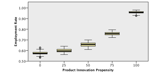
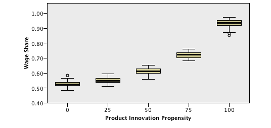
For more detail on the sensitiveness of output values to different parameter values, please refer to Appendix A.
Analysis of the dynamics of the economy
The present section contains charts depicting the evolution of the values of output variables throughout simulations. In order to achieve a compromise between comprehensiveness and simplicity of the results, only one initial parameter was considered as having more than one initial value: the Product Innovation Propensity. Indeed, this is the initial parameter with the most influence on the outcomes of the model. As such, two scenarios will be considered, one in which the Product Innovation Propensity is 25 and one in which it is 75, that is: one can expect more firms to be attempting Product Innovation in Scenario 2 than in Scenario 1 and more firms to be attempting Process Innovation in Scenario 1 than in Scenario 2.
In order to prevent the obtained values from being merely a result of the degree of randomness of the model, 10 iterations of each scenario were run, and the values presented are the average of the results of those 10 iterations, in each scenario, at each time step.
The gap between product and process innovation rates as a determining factor of the employment rate and wage share
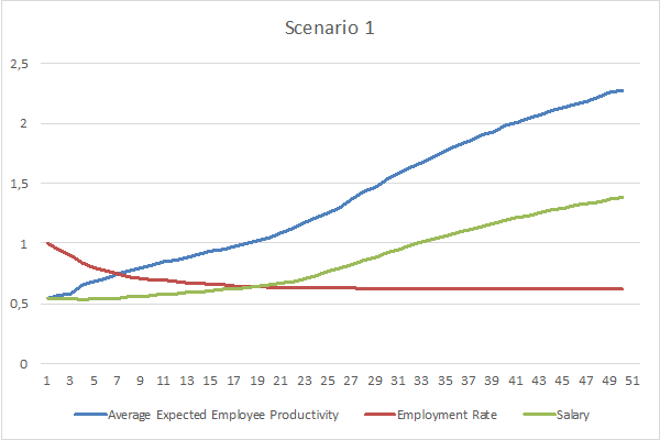
The following charts represent the evolution of the Employment Rate, Innovation Rates, and Wage Share in both Scenarios:
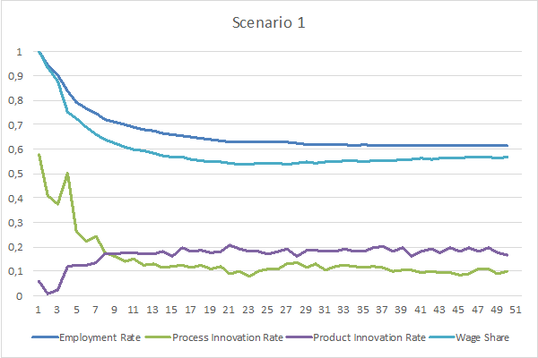
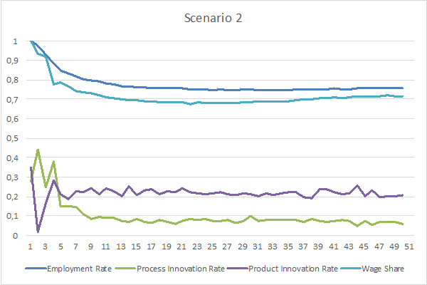
In both scenarios, Employment Rates and Wage Shares start decreasing until they stabilize around certain values. However, in Scenario 2, Employment Rate and Wage Share stabilize around 75% and 70% respectively, whereas in Scenario 1 they stabilize around 60% and 57% respectively. Additionally, Scenario 2 presents a larger gap between Product Innovation Rate and Process Innovation Rate than Scenario 1.
Regarding the evolution of Employment Rates, there appear to be two determining factors: the automation potential of tasks in the economy, and the gap between Product Innovation and Process Innovation Rates. The next two paragraphs attempt to explain the extent of influence of these factors.
Even considering a hypothetical modelling scenario in which firms performed absolutely no Product Innovation, but were able to perform Process Innovation to the point that every automatable tasks would be automated, some tasks would still be performed manually, because they were considered to be non-automatable. In this scenario, the percentage of manually performed tasks, and therefore the Employment Rate, would tend to match the percentage of non-automatable tasks in the economy, which is determined by the automation potential considered for the tasks in the economy.
In the presented model, the average automation potential of tasks in the economy is around 46%, meaning that 54% of tasks are considered to be non-automatable. However, both Scenario 1 and Scenario 2 present Employment Rates constantly above 54%. The reason for this is the fact that, unlike the hypothetical modelling scenario considered in the previous paragraph, firms in the presented model are able to perform Product Innovation instead of Process Innovation. Effectively, the charts appear to indicate that the gap between Product Innovation Rates and Process Innovation Rates influences the extent to which Employment Rates are higher than the proportion of non-automatable tasks in the economy.
The gap between product and process innovation rates as a determining factor of the gap between employee productivity growth and wage growth
The following charts represent the evolution of the Employment Rate, Expected Employee Productivity, and Salary in both Scenarios.
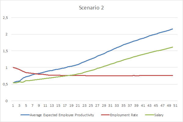
In both scenarios, the Average Expected Employee Productivity and the Salary keep increasing over time, while the Employment Rate decreases until it stabilizes. However, the Employment Rate stabilizes over a higher value in Scenario 2 than in Scenario 1 and, as a result, the gap between Average Expected Employee Productivity and Salary is larger in the first Scenario. It should also be noted that the Average Expected Employee Productivity is roughly equivalent over time in both Scenarios, even if slightly higher in Scenario 1.
Before drawing further conclusions, one must consider that process innovation exerts two opposing effects on the average salary. On one hand, process innovation increases the productivity of workers; while on the other hand, it decreases the demand for labour, thus diminishing workers’ bargaining power. In the simulations performed, the net effect of more process innovation (Scenario 1) was a lower average salary.
These results provide an additional explanation for the pattern of lower Wage Shares in Scenario 1 than in Scenario 2, as presented in Figure 1. Indeed, Wage Shares are lower in Scenario 1 not only because there’s a lower share of the population earning wages (since Employment Rates are lower), but also because the Employed Population earns as Salary a lower share of their productivity.
In this regard, it is important to mention that related phenomena have been observed in economies around the world in recent years. In fact, since the early 1980s, wage shares have significantly declined in the majority of countries and industries (Karabarbounis & Neiman 2014). Additionally, as Schwellnus et al. (2017) stresses, the last two decades, for the majority of OECD countries, were featured by a decoupling of aggregate labour productivity growth from real median compensation growth. Not surprisingly, these phenomena appear to be related, with Schwellnus et al.(2017) indicating that the decoupling of both growth rates is associated with both a decrease of wage shares and an increase of wage inequality. In its turn, Karabarbounis & Neiman (2014) indicate that about half of the decline in the global labour share can be explained by the decrease in the relative price of investment goods, such as information technology, which led firms to invest more heavily in capital rather than labour. As such, empirical data appears to support the conclusion that process innovation, driven by advancements in information technology, has led to a decline of wage shares and to a higher gap between productivity and wage growth, similarly to what one can observe in the performed simulations.
Concluding Remarks
Employment serves many functions in modern societies. It can be a means of survival, a vehicle of social mobility, a symbol of social validation, a tool for psychological well-being, or even a source of purpose. Indeed, employment is a fundamental socio-economical phenomenon, and attaining a better comprehension of how it can be affected is, therefore, of critical importance.
Bearing in mind the relevance of understanding the mechanisms influencing employment, the goal of this paper has been to study the relationship between innovation and employment by using an ABM methodology. The analysis led to three major conclusions, valid in the context of the model presented:
- The Employment Rate in a given economy is dependent on:
- the automation potential of the tasks in that economy, with a higher automation potential having a negative effect on employment;
- the type of innovation performed by firms in that economy, with Product Innovation having a positive effect on employment and Process Innovation having a negative effect.
- In a given economy, if firms’ propensity for product and process innovation, as well as the automation potential of their tasks, are stable over time, the Employment Rate in that economy will tend to stability over time.
- Higher levels of Process Innovation, and lower levels of Product Innovation, lead to a more intense decline of wage shares and to a wider gap between employee productivity growth and wage growth.
Taking into account these conclusions, it is particularly interesting to consider their implications regarding economic policy. Indeed, while policy-makers may have no control over the automation potential of the tasks in their economy, they can still influence the decisions of firms regarding the type of innovations they perform. As such, one could argue that, by putting into place a set of economic policies (such as, but not limited to, financial and tax incentives) aiming at encouraging Product Innovations instead of Process Innovations, policy-makers could have a positive effect on their economy’s employment levels.
Nevertheless, when in the context of the real world, these conclusions must be considered with some caution, due to certain limitations of the developed model, namely on the following assumptions: (i) the nature of product innovation, which considers that new tasks must be initially performed by humans; (ii) homogeneous employee skill sets and simple labour market dynamics; (iii) the nature of the aggregate demand for goods and services, which is considered to always match the aggregate supply.
Despite the recognizable limitations of this model, it still fulfils its purpose, which was that of developing and analysing an ABM which represents an effective way of studying the dynamics of innovation and employment. In fact, this model presents a detailed yet general representation of reality, in what concerns the relationship between innovation and employment, which is, in itself, innovative in economic literature. Additionally, the analysis of the model and of the data resulting from simulations did provide interesting and coherent insights regarding this economic puzzle. As such, the basic components of this model may reveal themselves to be useful for further investigations on these dynamics.
Some examples of potential future research paths, built on top of the presented model, include:
- Representing the possibility of fundamental technological breakthroughs, which would allow for the consideration of an increasing automation potential for the tasks in the economy, and its impact on the employment level.
- Representing employees with heterogeneous skill sets and tasks with different skill requirements. Such representation would in turn require a more complex and realistic representation of the labour market, accounting for different demands and different compensations for the labour of employees with different skill sets. This model would allow the study of the impact of innovation on the employment and remuneration levels across groups of workers with different skill sets.
- Representing consumption in a more complex and realistic way, taking into account the disposable income and preferences of each consumer. This way, the model would be able to propagate the effects of variations in wage share and income inequality back to the aggregate demand and, therefore, to the aggregate output. In such a model, it would be particularly interesting to study the overall implications of income inequality and of the introduction of a Universal Basic Income.
Appendix
A: Sensitiveness Analysis
This subsection presents an analysis of statistics obtained at the last time step of each simulation, with the goal of understanding the relationships among them and between them and the initial parameters.
The variables which will be analyzed are the following:
- Product Innovation and Process Innovation Rates Over Time: as previously mentioned, Product and Process Innovation Rates measure the percentage of firms in the economy that successfully performed product innovation, or process innovation, at a given time step. The suffix “Over Time” in these variables refers to the fact that they represent the average of the respective rates over every time step of the simulation. In addition to the effective innovation rates, some of the analysis in this section contain Innovation Attempts Rates and Innovation Success Rates, which measure, respectively, the percentage of firms that attempted a given type of innovation, and the percentage of the attempts which were successful.
- Employment Rate: the fraction of the Active population which is Employed at the last time step of the simulation, that is, the total number of Employees in all the firms in the economy divided by the Active population.
- Human share of input: the fraction of the total tasks performed, at the last time step of the simulation, which are performed by humans.
- Wage Share: the fraction of the total Output in the economy that has been distributed as Salaries, at the last time step of the simulation.
- Firm Replacement Rate Over Time: the average, over every time step of the simulation, of the percentage of firms in the economy that were replaced by a new firm at a given time step.
- Weighted average profit margin: the average profit margin of the firms in the economy at the last time step of the simulation, weighted by the firms’ revenues.
The reason why some of the statistics collected contain information only regarding the last time step is because these attributes, like the employment rate or the profit margins, are not independent from the results of previous time steps. That is, the value of these statistics at the last time step is the result of mechanisms which, to a great extent, build on top of the historical values for these statistics in the previous time steps. As such, the value for this statistics at the last time step represents the final value of an evolution over time.
On the other hand, the Innovation Rates and Firm Replacement Rates statistics contain information on the average over every time step because the mechanisms which determine their values at every time step do not rely on the historical values of these statistics in the previous time steps. That is, the value of these statistics at the last time step does not represent the final value of an evolution over time and is, indeed, unlikely to provide valuable information regarding the simulation. However, the average of the values of these statistics over every time step provides us with important information for characterizing the results in the simulation.
In order to obtain statistically relevant data from the simulations performed on the model, different values for some of the initial parameters of the model were set, and, for each possible combination of the initial parameters, a series of 10 iterations of the model were run.
From the initial parameters of the model, the following have been arbitrarily set to a single value, since it is logically clear, from the way the model was built, that they would have no influence on the results of the simulations:
- Number of firms: 100;
- Number of tasks in each generation: 1000;
- Number of tasks known by each firm: 10;
- Expected output quantity in the economy at the first time step: 100000;
- Interest rate: 5%.
On the other hand, the following parameters have been assigned a set of different possible values:
- R&D Intensity: {0.25; 0.5; 0.75};
- Expected Growth: {0; 0.02; 0.1};
- Product Innovation Propensity: {0; 25; 50; 75; 100};
The following is a reiteration of the definition of these parameters:
R&D Intensity: this parameter defines the percentage of earning that each firm will invest in R&D at each time step. Since it is an attribute of the environment, and not of each specific firm, it is, as previously mentioned, equal for every firm. It should also be noted that this parameter remains constant throughout the different time steps of the simulations.
Expected Growth: refers to the expected growth rate of the total output units in the economy. The total expected output units in the economy influences the planned production of the firms. It should also be noted that this parameter remains constant throughout the different time steps of the simulations.
Product Innovation Propensity: at each step, each firm chooses one of the two types of innovation to perform, so this parameter, ranging from 0 to 100, influences their propensity to choose product innovation over process innovation. Since it is an attribute of the environment, and not of each specific firm, it is equal for every firm. It should also be noted that this parameter remains constant throughout the different time steps of the simulations.
As a result of running 10 iteration for each possible combination of initial parameters, a total of 450 simulations of the model were run.
In order to assess whether or not the values for the initial parameters have a significant effect on the values of the output statistics, a series of Kruskal-Wallis tests were performed. The Kruskal-Wallis test verifies the hypothesis that the distribution of a variable is the same across different independent samples. Being a non-parametric test, it does not rely on the assumption that the variable must be normally distributed, unlike the ANOVA method.
The goal was therefore to test whether the distribution of each output variable was the same across the different possible values of each initial parameter (Expected Growth, R&D Intensity, and Product Innovation Propensity).
The following is the SPSS output from the Kruskal-Wallis tests across values of Expected Growth:
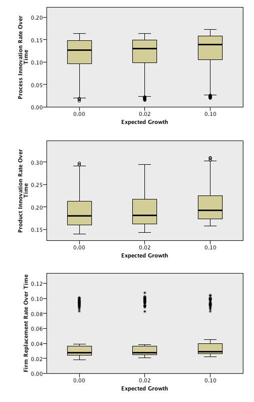
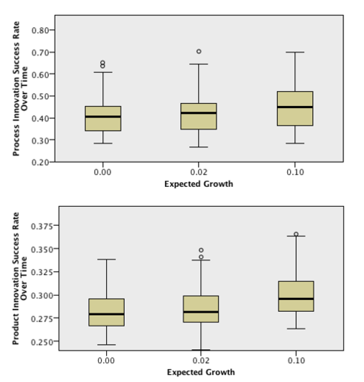
From this output, we can conclude with a significance level of 5% that Innovation Rates and Firm Replacement Rate Over Time present different distributions across the different values of Expected Growth. The following outputs are the boxplots of these variables across the different categories of Expected Growth:
From these outputs, it is possible to see that both the Product and Process Innovation Rates present distributions with higher values when the Expected Growth presents its highest value. Regarding the Firm Replacement Rate Over Time, it also appears to present a distribution with higher values for the last category.
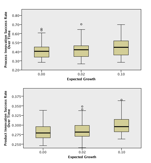
The fact that the distributions for both Innovation Rates present higher values can only be explained by higher Innovation Success Rates when the Expected Growth is higher. In fact, the sum of the two Innovation Attempt Rates is always 100%, so it would be impossible to see an increase in both Attempt Rates at the same time. In order to confirm the previous affirmation, the boxplots for both Innovation Success Rates are presented below:
As expected, both Innovation Success Rates present a distribution with higher values when the Expected Growth is the highest. Nevertheless, this result raises the question of why would Success Rates be higher under these circumstances. Indeed, this appears to be the result of the fact that relative R&D Stocks, which are the only determinant of the Innovation Success Factors, are computed by taking into consideration the average R&D Stock in the previous time step and, therefore, a higher growth of a firm’s revenues from one period to another may lead to a higher relative R&D Stock, since it may lead to a higher increase of profits and, therefore, to a higher increase of R&D Stocks. As such, this appears to be the result of the model configuration, rather than a result from which one can draw valid economic conclusions.
The following is the SPSS output from the Kruskal-Walis tests across values of R&D Intensity:
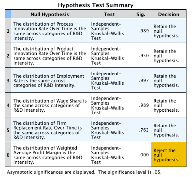
From this output, we can conclude with a significance level of 5% that the Weighted Average Profit Margin presents different distributions across the different values of R&D Intensity. The following output is the boxplot of this variable across the different categories of R&D Intensity:
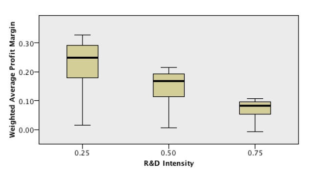
As it is clear to see, for higher values of R&D Intensity, the distributions of the Weighted Average Profit Margin present lower values. This result is expected and intuitive, considering that the R&D Intensity determines a firm’s R&D Expenses, which affects its Profit Margin.
It is also not surprising that we cannot reject the hypothesis that the Firm Replacement Rate Over Time is not different across different values of R&D Intensity, since firms only incur in R&D Expenses if their Revenues net of Production Costs are positive. That is, R&D Intensity may affect how high a firm’s net profitability is, but it doesn’t affect whether it is positive or negative.
The following is the SPSS output from the Kruskal-Walis tests across values of Product Innovation Propensity:
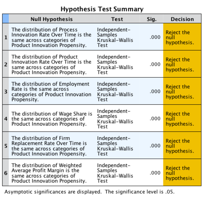
From this output, we can conclude with a significance level of 5% that all the output variables present different distributions across the different values of Product Innovation Propensity. The following outputs are the boxplots of each variable across the different categories of Product Innovation Propensity:
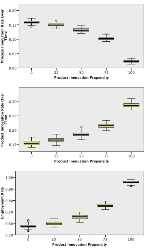
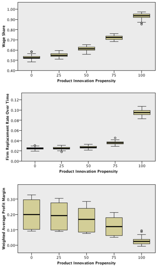
Once again, these results are not surprising. Product Innovation Propensity is highly determinant of both Product and Process Innovation Rates, and, as a result, of the other output variables. In fact, these results are coherent with the previously seen results on the correlations between Innovation Rates and the remaining output variables.
B: Model Programming Code
The present ABM was developed in Python, using the Mesa framework (Masad & Kazil 2015).
References
AGHION, P. & Howitt, P. (1994). Growth and unemployment. The Review of Economic Studies, 61(3), 477-494.
AXELROD, R. & Tesfatsion, L. (2005). 'A guide for newcomer to agent-based modeling in the social sciences.' In L. Tesfatsion & K. Judd (Eds.), Handbook of Computational Economics, Vol. 2,. Amsterdam: Elsevier, pp. 1647–1659.
BOUCHAUD, J-P. (2008). Economics needs a scientific revolution. Nature 455(7217), 1181.
DAWID, H. (2006). 'Agent-based models of innovation and technological change.' Handbook of Computational Economics, Vol 2. Amsterdam: Elsevier, pp. 1235–1272.
DECANIO, S. J. (2016). Robots and humans – Complements or substitutes? Journal of Macroeconomics, 49, 280-91.
FAGIOLO, G., Dosi, G. and Gabriele, R. (2004). Matching, bargaining, and wage setting in an evolutionary model of labor market and output dynamics. Advances in Complex Systems, 702), 157-186.
FAGIOLO, G. and Roventini, A. (2017). Macroeconomic policy in DSGE and agent-based models. Journal of Artificial Societies and Social Simulation, 20(1), 1: https://www.jasss.org/20/1/1.html.
FARMER, J. D. & Foley, D. (2009). The economy needs agent-based modelling. Nature, 460(7256), 685.
FORD, M. (2015). Rise of the Robots: Technology and the Threat of a Jobless Future. New York, NY: Basic Books.
GRIMM, V., Augusiak, J., Focks, A., Frank, B. M., Gabsi, F., Johnston, A. S. A., Liu, C., Martin, B. T., Meli, M., Radchuk, V., Thorbek, P., & Railsback, S. F. (2014). Towards better modelling and decision support: Documenting model development, testing, and analysis using TRACE. Ecological Modelling, 280, 129-139.
GRIMM, V., Berger, U., DeAngelis, D. L., Polhill, J. G., Giske, J., & Railsback, S. F. (2010). The ODD protocol: A review and first update. Ecological Modelling, 221(23), 2760–2768.
GRIMM, V., Polhill, G, & Touza, J. (2013). Documenting social simulation models: The ODD protocol as a standard. In B. Edmonds & R. Meyer (Eds.), Simulating Social Complexity: A Handbook. Berlin/Heidelberg: Springer, pp. 117-133.
GRIMM, V. & Railsback, S. F. (2012). 'Designing, formulating, and communicating agent-based models.' In A.J. Heppenstall, A.T. Crooks, L.M. & M. Batty (Eds.), Agent-Based Models of Geographical Systems. Springer: Dordrecht, pp. 361-377.
JANSSEN, M., Alessa, L. N., Barton, M., Bergin, S, & Lee, A. (2008). Towards a community framework for agent-based modelling. Journal of Artificial Societies and Social Simulation, 11(2), 6: https://www.jasss.org/11/2/6.html.
KARABARBOUNIS, L. & Neiman, B. (2014). The global decline of the labor share. The Quarterly Journal of Economics, 129(1), 61–103.
MANYIKA, J., Chui, M., Miremadi, M., Bughin, J., George, K., Willmott, P., and Dewhurst, M. (2017). A future that works: automation, employment, and productivity. McKinsey Global Institute (January 2017).
MASAD, D. & Kazil, J. (2015). MESA: An agent-based modeling framework. In Proceedings of the 14th Python in Science Conference (SCIPY 2015), pp. 53-60.
NETO, A. & Silva, S. T. (2013). Growth and Unemployment : A bibliometric analysis on mechanisms and methods. FEP Working Papers, 498 (July 2013).
SAFARZYŃSKA, K. & van den Bergh, J. C. J. M. 2010. “Evolutionary Models in Economics: A Survey of Methods and Building Blocks.” Journal of Evolutionary Economics 20(3), 329-73.
SCHUMPETER, J. A. (1943). Capitalism, Socialism and Democracy. London: Allen and Unwin.
SCHWELLNUS, C., Kappeler, A., & Pionnier, P.-A. (2017). Decoupling of wages from productivity: Macro-level facts.” OECD Economics Department Working Papers, 1373.
SILVA, S. T. (2009). On evolutionary technological change and economic growth: Lakatos as a starting point for appraisal. Journal of Evolutionary Economics, 19(1), 111-35.
SILVA, S. T., Valente, J. M. S., & Teixeira, A. A. C. (2012). An evolutionary model of industry dynamics and firms’ institutional behavior with job search, bargaining and matching. Journal of Economic Interaction and Coordination, 7(1), 23-61.
STARE, M. & Damijan, J. (2015). Do innovation spillovers impact employment and skill upgrading? The Service Industries Journal, 35(13), 728-745.
TESFATSION, L. (2016). Presentation and evaluation guidelines for Agent-Based Models. Retrieved January 13, 2017: http://www2.econ.iastate.edu/tesfatsi/amodguide.htm.
VIVARELLI, M. (2014). Innovation, Employment and Skills in Advanced and Developing Countries: A Survey of Economic Literature. Journal of Economic Issues, 48(1), 123-154.