An Integrated Ecological-Social Simulation Model of Farmer Decisions and Cropping System Performance in the Rolling Pampas (Argentina)

, ,
and
aUniversidad de Buenos Aires, Argentina; bCONICET-Universidad de Buenos Aires. Instituto de Investigación en Ciencias de la Computación, Argentina
Journal of Artificial
Societies and Social Simulation 25 (1) 5
<https://www.jasss.org/25/1/5.html>
DOI: 10.18564/jasss.4772
Received: 28-Dec-2019 Accepted: 26-Dec-2021 Published: 31-Jan-2022
Abstract
Changes in agricultural systems are a multi-causal process involving climate change, globalization and technological change. These complex interactions regulate the landscape transformation process by imposing land use and cover change (LUCC) dynamics. In order to better understand and forecast the LUCC process we developed a spatially explicit agent-based model in the form of a Cellular Automata: the AgroDEVS model. The model was designed to project viable LUCC dynamics along with their associated economic and environmental changes. AgroDEVS is structured with behavioral rules and functions representing a) crop yields, b) weather conditions, c) economic profits, d) farmer preferences, e) adoption of technology levels and f) natural resource consumption based on embodied energy accounting. Using data from a typical location of the Pampa region (Argentina) for the period 1988-2015, simulation exercises showed that economic goals were achieved, on average, each 6 out of 10 years, but environmental thresholds were only achieved in 1.9 out of 10 years. In a set of 50-years simulations, LUCC patterns converge quickly towards the most profitable crop sequences, with no noticeable trade-off between economic and environmental conditions.Introduction
In agroecosystems, land-use and cover change (LUCC) is driven by simultaneous responses to economic opportunities, institutional factors and environmental constraints (Lambin et al. 2001). Different methodological approaches are used for assessing LUCC by capturing the dynamic process influenced by complex interactions between socio-economic drivers and biophysical conditions. For example, the spatially explicit LUCC models assess location suitability for different land uses and allocate changes to grid cells based on suitability maps (Verburg, de Nijs, et al. 2004). Another modelling approach has been developed for capturing the behavior of the real actors of land-use change: individuals and/or institutions (“agents”) become the objects of analysis, modelling and simulation, paying explicit attention to interactions between these agents of change (Castella & Verburg 2007). In this modelling approach, farmers’ responses to environmental, economic and sociological constraints for deciding on LUCC are crucial for assessing the agricultural system sustainability. Such models are known as agent-based models (ABM).1
The ABM approach provides a flexible paradigm for studying emergent patterns in complex systems (Cook 2009). Particularly, in agricultural systems the ABMs are capable of capturing the individual agent behavior in response to several constraints scenarios (e.g., climate, socio-economical). In addition, it is possible to develop ABMs into spatially explicit frameworks for exploring the LUCC process over time. Examples may include spatial interaction models, cellular automata (CA) and dynamic system models (Evans & Kelley 2004). However, when ABM are used to cope with complex systems the development of models often tends to get forced to the ABM paradigm even when certain dynamics are not necessarily well expressed in the ABM realm. In this context, the Discrete Event Systems Specification (DEVS) modelling and simulation framework (Zeigler et al. 2000) offers a universal paradigm for modelling hybrid models (continuous, discrete time, discrete event) that are able to scale up through the interconnection of models of very different nature, including the ABM approach. In the case of environmental systems there exists a considerable modelling experience based on the DEVS formalism (Filippi et al. 2010). Notably, when ABM needs to be combined with spatially explicit dynamics, the Cell-DEVS formalism provides means to attain this goal within the DEVS framework (see Wainer (2006) and Kazi & Wainer (2018) for experiences on Cell-DEVS applied to environmental dynamics). DEVS enforces the formal specifications and strict separation between model specification, abstract simulator algorithm, and experimental framework. This greatly facilitates modelling and simulation software development efforts, as modelling, simulation and experimentation techniques can progress in parallel but along independent paths, preserving their composability into integrative solutions. For instance, Zapatero et al. (2011) developed a DEVS-based software solution where GIS technology, Cell-DEVS models, DEVS distributed simulation and Google Earth visualization were orchestrated to build a fire spread simulation application relying on pre-existing components. More background on applying DEVS to express ABMs in the simulation of artificial societies can be found in Lee et al. (2015); Yun & Moon (2020); Yun et al. (2015).
Although the ABM approach is widely used to explain land use change and future policies impacts, the development of LUCC simulation models coupled with environment impact assessment is still incipient in agricultural systems (Kremmydas et al. 2018). The first generation of ABM was related to agricultural economics (Balmann 1997), followed by several studies to simulate the performance of individual farms and their spatial interactions (Berger 2001; Happe et al. 2008; Schreinemachers et al. 2007). It has been recently recognized that the incorporation of material and energy flows during land-use conversion are increasingly needed to explore socio-economic dynamics and land-use change (Lee et al. 2008). Some ABMs also include other aspects such as policy implications (Happe et al. 2006), environmental processes (Schreinemachers & Berger 2011), or organizational and market dynamics (Bonabeau 2002).
In this work we study the Pampa region in Argentina, which in the last decades went through an agricultural intensification process that led to an expansion of the area sown with soybean, replacing pastures and perennial crops (A. 2009; Paruelo et al. 2005). Although this landscape homogenization was accompanied by an immediate economic benefit, it also exacerbated social, environmental and economic impacts of the agricultural systems. In the Pampa region, where climate, technological innovations, and socio-economic contexts affect agricultural production, the ABM approach for LUCC modelling has not been frequently addressed (Groeneveld et al. 2017). An exception is the model of Bert et al. (2011) (the PAMPAS model) designed to gain understanding about both structural and land use changes in the Pampas. Although we use a modelling approach similar to the PAMPAS model in terms of agent behavior, PAMPAS does not include any modelling effort to assess the status level of natural resources affected by the LUCC simulated process (in the work of García et al. 2019 it was used to capture linkages at the climate/water/crop nexus in the Argentine Pampas).
In this work, we developed an ABM model called AgroDEVS, implemented with the Cell-DEVS cellular automata-oriented formalism that relies on the Discrete Event Systems Specification (DEVS) modelling and simulation framework. The goal of AgroDEVS is to integrate into a single model the main driving forces (i.e., climate, agronomic management, and farmer decisions) for explaining LUCC as well as the environmental and economic consequences of these changes. This integration is developed into a decision-making tool that can be extended and improved to specific policy contexts. AgroDEVS aims to simulate LUCC as well as economic profit and fossil energy use (as a proxy of the environmental condition), both at the individual (agent) and collective (landscape) scales.
Materials and Methods
Region under study and cropping system description
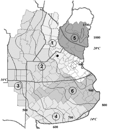
AgroDEVS was applied to simulate LUCC dynamics in Pergamino, a typical location in the Rolling Pampas (Figure 1), the most productive subregion of the Pampas where most of the annual cropping is concentrated (Hall et al. 1992). The Pampa is a fertile plain originally covered by grasslands, which during the 1900s and 2000s was transformed into an agricultural land mosaic by grazing and farming activities (Soriano et al. 1991). The predominant soils are typical Arguidols and the annual rainfall averaged 950 mm (Moscatelli et al. 1980). AgroDEVS simulates LUCC using the most frequent crop types in the Pampa region (Manuel-Navarrete et al. 2009): (1) the wheat/soybean double-cropping (\(W/S\)); (2) maize cropping (\(M\)), and spring soybean cropping (\(S\)). In this paper, the terms "crop"; “crop type” and "land use" (i.e. cropping systems) were used interchangeably as well as “farmer” and “agent”. The agronomic decisions (i.e. genotype selection, fertilizer management, pest control, sowing date, and soil type) were representative of the most frequent situation for each of the cropping systems.
Cellular Automata-based modelling and simulation approach
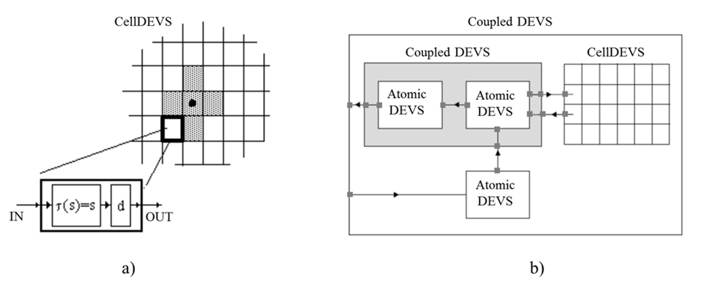
For the modelling activity we followed a scenario-based analysis, exploring agricultural mosaic dynamics. Then we adopted an agent–based modelling (ABM) approach, by identifying both landscape and agent-specific descriptors as parameters (fixed) or attributes (variable). We defined parameters as any fixed condition for describing the behavior or the condition of a model element. On the other hand, the attributes represent the system changes during the model run period. Lastly, we adopted a formal model-based simulation framework to specify mathematically both the parameters and attributes due to different behaviors. For this purpose, we encoded AgroDEVS using the Cell-DEVS formalism. Cell-DEVS is an extension for Cellular Automata of the more generic Discrete EVent System Specification (DEVS) formal modelling and simulation framework. On the one hand, the DEVS formalism permits to express and combine any kind of dynamical system (continuous, discrete event, discrete time) in a mathematical form that is independent of any programming language. On the other hand, Cell-DEVS provides the modeler with a meta-language tailored to facilitate the expressing of systems where the spatial arrangement of “cells”, and their behavior, plays a key role. By adopting the DEVS-based approach, AgroDEVS becomes readily linkable with other DEVS models developed by others for different domains (e.g. climate, biology, sociology, and economics), potentially using heterogeneous techniques (e.g. differential equations, equilibrium models, optimization models, stochastic processes). In Figure 2 we summarize these concepts. Atomic DEVS are the smallest units of behavior. They can be interconnected modularly through input and output ports to compose hierarchies of more complex systems called Coupled DEVS (Figure 2b). Cell-DEVS features an automatic composition of Atomic DEVS models in the form of an \(N\)-dimensional lattice. Each cell gets interconnected only to other cells belonging to a neighborhood shape defined by the modeler (Figure 2a). Cell-DEVS features a rule-based compact language to model the behavior of each cell in relation to its neighborhood, influencing each other.
Behavioral rules are used in the Cell-DEVS language to define the change of attributes that are local to each cell. These variables can express properties for that unit of space (e.g., in the 2-dimensional case it can be an agricultural plot). When the modeler uses such variables to express also the attributes of “agents” located at cells, then the ABM approach can be merged into the system. In the case of AgroDEVS each agent (namely, a farmer) remains fixed to his or her plot, and rules are used to express changes both for the physical environment and the for farmer, which eventually affect each other. In this work, we adopted the CD++ simulation software toolkit, which is capable of interpreting Cell-DEVS and DEVS models and of simulating them. CD++ implements a generic DEVS “abstract simulator”, consisting of a standardized algorithmic recipe that specifies how to simulate any DEVS model independently of any programming language of choice. We believe this generic, reusable and extensible DEVS-based approach provides AgroDEVS with very desirable scalability and sustainability features. The full model represents the collective (i.e., landscape-level) function that emerges from the aggregation of all farmers’ outcomes. It also depends on exogenous variables (e.g., climate, crop (output) prices, and production costs) as well as endogenous variables (e.g., the farmer’s technological level, the outcomes of neighboring farmers, and each farmer’s performance history). The model proved particularly well suited to reproduce empirical situations where (a) there are changes in the relative production/output prices between potential land uses, (b) there is a specific climate regime that impacts on crop yields, or (c) there are varying aspiration levels for the farmers (Gotts & Polhill 2009).
In Appendix E we provide more technical details about the model specification approach, its modelling language, rule specification, simulation framework and experimentation environment.
Model verification, validation and sensitivity analysis
We submitted AgroDEVS to a systematic verification and validation process (Wilensky & Rand 2007). Firstly, a code walk-through (Stern 2003) was performed to review the model formulation and to ensure that all design concepts and specifications are correctly reflected in the code. In addition, AgroDEVS was run with very few farmers in the grid (9-16) and results were examined closely (e.g., following dynamics of specific farmers, inspecting the outliers). The intrinsic complexities and uncertainties on both the magnitude and the nature of the forces driving land use change, lead to expanding the scope of the straightforward evaluation between simulated and observed patterns in the model validation phase (Bert et al. 2014; Le et al. 2012; Nguyen & de Kok 2007). Our model development process seeks to validate the ABM through a process of continuous adaptation using feedback from the stakeholders (Ligtenberg et al. 2010). Specifically, AgroDEVS development entailed a continual discussion process with stakeholders (data not shown) from the study area in order to review both the rules and the assumptions of the model that initially came from the literature review. This approach directly engages stakeholders in model development by embedding it within the social process of policy development (Moss 2008). This changes the validation problem into an advantage: the agreement of participants or stakeholders may be an indicator of the validity of a simulation model (Troitzsch 2004). In AgroDEVS, the evaluation of the simulation is guided by the expectations, anticipations, and experience of the community that uses it for practical purposes (Ahrweiler & Gilbert 2005), and this supports the view that the very meaning of validity is dependent on the purpose of the simulation models under examination (Küppers & Lenhard 2005). Moreover, it is possible to develop a model that fits the data perfectly with a model structure that does not capture any real processes (Cooley & Solano 2011). Due to the complex nature of ABMs (e.g., nonlinear responses to parameters) a broad single-parameter SA (Appendix A) was performed (Railsback & Grimm 2015). This type of analysis assesses the effect of each parameter over a wide range of values, as opposed to the traditional local analysis, in which each model input is varied by a standard small amount (Ligmann-Zielinska et al. 2020; Railsback & Grimm 2015). The goodness-of-fit of each simulated LUCC was calculated using 1) Normalized RMSE: \(v = RMSE/Observed \; mean\; \% Total\; area\); 2) Probability of a Match: \(PM = \#matches / (\#matches + \#mismatches)\); and 3) Index of Observed Fit: \(IOF = (2 \times PM) - 1\).
\(PM\) are the chances that a simulation can correctly predict the order of any pair of observations. The number of matches (#matches) is calculated by counting the set of ordered pairs of observations that match the predicted ordered pairs of a simulation (Thorngate & Edmonds 2013). \(IOF\) is an index that derives from the calculations of the PM. Its values range from \(IOF = +1\) (all observations match predictions), through \(IOF = 0\) (half of the observations match), to \(IOF = -1\) (none of the observations match predictions).
Results
Model description
The model description follows the ODD protocol “ODD” (Overview, Design concepts, and Details) to standardize the published descriptions of individual-based and agent-based models (Grimm et al. 2010). We describe in the following subsections 1) the model’s purpose, 2) the system variables and 3) the process overview to emphasize the main message of the model outputs. The remaining items of the ODD protocol (initialization conditions, submodels description, input data, modelling approach, and design concepts) can be found in the Appendixes B to F.
Model’s purpose
The main modelling purposes (see Edmonds 2017) of AgroDEVS are 1) Prediction, as there is a need to be able to anticipate aspects of the agricultural system that are not currently known; and 2) Explanation, as the model tries to identify the causal interactions between the main driving forces of LUCC phenomena (prediction alone does not provide insights on the internal dynamics driving the evolution of system processes).
System variables
AgroDEVS maps farmers onto a regular grid in order to initialize the simulations. The model consists of two entities: 1) the landscape and 2) the agents that operate on the landscape. Each entity has its own set of fixed parameters and attributes that evolve throughout simulation cycles. The landscape parameters are a) the number of agents and b) the owner/tenant agent ratio and the landscape attribute is the overall outcome from the integration of all individual agent attributes results within the simulated landscape. The agent parameters are a) the land rental price (\(RP\)) for the tenants, and b) its location on the grid. The attributes for each agent are a) the technological level (\(TL\)), b) the crop type allocation (or land use, \(LU\)), c) the economic profit (\(P\)), d) the renewability level (\(RL\)) of the embodied energy (emergy) consumption (see Appendix C Renewability level calculations section for an emergy concept explanation), e) the aspiration level (\(AL\)), f) the environmental threshold (\(ET\)), and g) the weather growing condition (\(WGC\)).
Process overview
AgroDEVS simulations advance with an annual time step, representing a single cropping cycle (\(CC\)) (Figure 3). Crop yields under different WGC were previously simulated (Appendix B, Table 2) using the DSSAT model (Jones et al. 2003). We used local management data for defining resource level in each \(TL\) (e.g., fertilization regime, genotype) as well as five contrasting historical weather records for defining the different \(WGC\) levels.
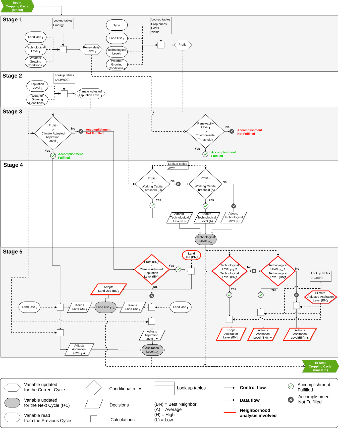
At the start of the AgroDEVS simulation process (Figure 3, Stage 1), each initial agent’s configuration (\(LU_{t}\)) is exposed to a climate-related growing condition level \(WGC\) that ranges from very favorable to very unfavorable for high crop yield achievement. Then, based on 1) the previously simulated crop yields, 2) the crop price, 3) the production cost of each \(TL\), 4) the land rental price and 5) the crop type allocation into the farm household, AgroDEVS calculates the farmer’s \(P_{t}\): the profit \(P\) for the current time \(t\), or similarly, for the current cropping cycle \(CC\). At this first step, AgroDEVS also calculates \(RL_{t}\) (see Appendix C for \(RL\) calculation details) as a measure of the renewable energy consumption of the cropping cycle. At the next stage, the initial agent’s aspiration level (\(AL_{t}\)) is adjusted by means of the current \(WGC_{t}\) level resulting in a new climate-adjusted aspiration level (\(CAL_{t}\)) (Figure 3, Stage 2). Then, AgroDEVS uses \(P_{t}\) and \(RL_{t}\) values calculated in Stage 1 for assessing the fulfillment of both the environmental (\(ET\)) and economic (\(AL\)) goals (Figure 3, Stage 3) of each agent. An agent will keep its crop type allocation once the \(P_{t}\) value is greater than or equal to its \(CAL_{t}\) at each \(CC\), while non-fulfillment of environmental threshold (\(ET\)) does not alter its crop type allocation decision. AgroDEVS assesses whether the farmer can upgrade or downgrade its \(TL\) for the next \(CC\), according to their economic performance in the current \(CC\) (Figure 3, Stage 4). For this adjustment, AgroDEVS defines a set of different working capital thresholds (\(WCT\)) in order to access different \(TL\) values. The \(WCT\) fulfillment is assessed using \(P_{t}\). If \(P_{t}\) is lower than the respective \(WCT\), the farmer must lower its \(TL\) (and vice versa). Eventually, agents can remain at the lowest \(TL\), regardless of its \(P_{t}\) value (i.e., no agent is forced out of business). During this stage, AgroDEVS also adjusts the farmer’s aspiration level (\(AL\)) for the next \(CC\). This setting is based on a) the farmer’s perception of the \(WGC\) level of the next \(CC\), and b) the agent’s failure or success at achieving the \(AL\) in the previous \(CC\), respectively. Values of 1) crop prices, 2) adjustment factor of the aspiration level due to \(WGC\), 3) adjustment factor of the aspiration level due to \(TL\), and 4) working capital threshold for \(TL\) are shown in the Appendix B, Tables 4 to 7, respectively).
Simulation results for Pergamino 1988-2015
LUCC patterns
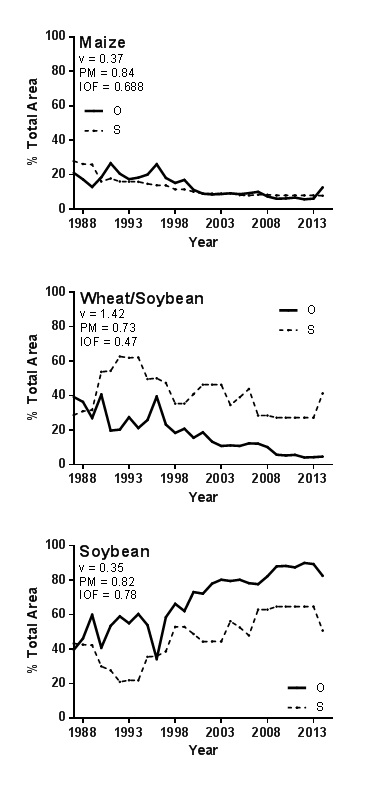
The simulated LUCC patterns replicated the overall trend towards soybean-dominated landscapes observed in the region since the mid-1990s. The ordinal pattern analyses (OPA) showed a similar, relatively high \(PM\) for maize, wheat/soybean, and soybean, evidencing the model’s capability to predict ordinal (higher/lower) values of crop type cover. However, the accuracy in predicting the magnitude of these changes was lower (Figure 4). Based on the RMSE method, the goodness-of-fit of the wheat/soybean simulated cover was the lowest among the three-crop types, resulting in a significant overestimation of this cropping area. The model underestimated simulated soybean cover. In addition, the \(v\) values (i.e., the RMSE relative to the observed mean) was remarkably higher for wheat/soybean than in both maize and soybean.
Profit, renewability, and technological levels
Profit (\(P\)) and renewability level (\(RL\)) values for the Pergamino simulation correlated without any significant trend throughout the study period (Figure 5). Remarkably, in only four years of the simulated period, the simulated landscape exhibited higher \(RL\) values than the ecological threshold (\(ET > 50\% RL\)). Inter-agent variability in the simulated landscape depicted a range of decisions (in terms of crop type allocation) that resulted in a great variability on average \(P\) values during the simulation (Figure 6, Panel A).
The interquartile \(P\) range (25–75% percentile) varied between 94 and 556 US$/ha (Figure 6, Panel A). However, the \(RL\) interquartile range was not as high as the observed in \(P\) (Figure 6, Panel A). The relative homogeneity between each cropping production system, in terms of external inputs, generated a remarkably low variability in \(RL\) terms during the whole simulated period. In this case, the interquartile \(RL\) range varied from 37.9% to 43.5% with a median value of 41.2%, almost ten percentage points lower than the environmental threshold (\(ET\)) of 50% (Figure 6, Panel A). While in terms of \(RL\), the variability between agents was significantly lower than those observed for \(P\), it was possible to detect both maximum and minimum \(RL\) values showing the model capability to simulate a wide area of decisions during the simulated period. Minimum average value for an agent outcome in terms of \(RL\) was 29% and the maximum \(RL\) average value for an agent was 49.4% (Figure 6, Panel A), a condition of very close agreement with the environmental threshold (\(ET\)). Agent behavior in AgroDEVS was also assessed by inspecting the intra-agent variability, using both \(P\) and \(RL\) during the simulation period (Figure 6, Panel B). The interannual coefficient of variation of \(P\) showed a median value of 57%, with an interquartile range between 49.8% and 264.5% (Figure 6, Panel B). The \(RL\) interannual variation was significantly lower than \(P\), exhibiting a median coefficient of variation of 18.9% and an interquartile range between 16% and 22% (Figure 6, Panel B).
An assessment of the simulation results was carried for both the environmental (\(ET\)) and economic (\(AL\)) goal agreements exhibited by agents throughout the simulation period (Figure 6, Panel C). The goal agreement metric indicates the percentage of years during which an agent fulfills each of the goals (environmental and economic). The agents exhibited an interquartile range of economic (\(AL\)) goal agreement between 32% and 64% with a median of 60% and maximum and minimum of 71.4% and 17.2%, respectively (Figure 6, Panel C). These values are noticeably higher than the \(RL\) goal agreement that showed a median of 17.9% with an interquartile range between 7% and 25% (Figure 6, Panel C). The agent’s capability for adjusting the \(AL\), based on both the current climate condition (\(WGC\)) and the \(AL\) fulfillment in the previous agricultural cycle, could explain the better goal agreement when compared against \(RL\), which is a fixed parameter. When inspecting the extreme values for \(RL\) goal agreement, it was possible to identify a single agent exhibiting a maximum value of 46.4%. This means that, under the same economic and climate conditions, this agent was able to fulfill nearly 1 out of 2 years the \(RL\) threshold (\(ET\)) by means of its crop type allocation decisions.
Lastly, the model outcome was also assessed by inspecting the final distribution of the three different technological levels (\(TL\)) across all 625 agents of the Pergamino simulation (Figure 7). The closely related observed and simulated agent distribution underline the model’s ability to represent the process of agricultural intensification evidenced by a higher proportion of farmers using a technological level with higher levels of inputs. Both observed and simulated \(TL\) distribution patterns exhibit a dominance of the high \(TL\). However, the model retains a greater percentage of agents at the lowest level (\(TL\) low) than in the observed data. It is possible that the model structure, which allows agents to remain using the lowest \(TL\) despite not reaching the minimum wealth to face those costs, is an explaining factor for the overestimation of Low \(TL\) at the end of the simulation.
Long-term scenarios
LUCC patterns
The objective of the long-term simulations was to assess the magnitude of the effect of the tenure condition (i.e., an owner or tenant-dominated landscape) and climate (i.e., five contrasting climate regimes) on both LUCC (Figure 8), and \(P\) and \(RL\) outcomes (Figure 9). AgroDEVS simulations showed that the variability in climate regimes altered the pattern of crop type dominance at the end of the simulation cycles (Figure 8). In terms of LUCC, under constant climate regimes (Figure 8: L, A and H Panels) the simulated landscape is always stabilized at higher values of soybean (\(S\)) cover, followed by the wheat/soybean double-cropping (\(W/S\)) and maize (\(M\)). On the other hand, under variable climate scenarios (Figure 8: V and R Panels) the long-term simulations showed the highest crop type dominance represented by \(W/S\) instead of \(S\), although \(M\) remained at the lowest cover throughout the simulated period. Tenure effect on LUCC dynamics was clearer under constant average climate regime (Figure 8: Panel A; 10O/90R). Under this scenario, the landscape dominated by tenants exhibited a much stronger \(S\) dominance, compared to \(W/S\) or \(M\). Instead, under the same climate scenario but dominated by owners (Figure 8: Panel A; 90O/90R), the model simulated a different LUCC dynamic, showing an earlier stabilization point for LUCC (ca. year 2) and very similar final cover values for the three analyzed crop types. Oppositely, the model showed similar LUCC dynamics in owners or tenants-dominated landscapes, under a constant unfavorable (Figure 8: Panel L) and constant favorable (Figure 8, Panel H) climate regimes. In variable climate scenarios, the regular see-saw climate change pattern (Figure 8, Panel V) showed less differences in LUCC pattern due to land tenure regimes with respect to the random climate pattern (Figure 8, Panel R). The inclusion in the simulation scenario of climate dynamics without a definite pattern (i.e., random) resulted in the increase of double cropping \(W/S\) dominance, and this effect was much stronger for the condition of a landscape dominated by owners, achieving in this condition the highest crop type dominance among the 10 long-term scenarios (Figure 8: Panel R; 90O/10R).
Profit and renewability level
The variability between long-term scenarios was lower for both \(P\) and \(RL\) than for the simulated LUCC (Figure 9). Regarding the variability induced by the climate regime, the simulated landscapes were stabilized at increasing \(P\)-values, as climate scenarios were better (Figure 9: Panels L, A, and H). This effect of profit improvement occurred in both tenant- and owner-dominated landscapes. In this latter case, the stabilized \(P\) values were due to the differential income associated with non-payment of land rental.
Although the simulated landscape configurations were clearly different (Figure 9), the \(RL\) variability among long-term scenarios under constant climate regimes (when stabilized) showed very small changes (less than 10%) between the maximum and minimum \(RL\) final values (Figure 9, Panels L, A, V). When analyzing the scenarios under variable climate regimes (Figure 9, Panels V; R) a regular pattern of both \(RL\) and \(P\) variations was observed when climate evolved in a regular way (Figure 9, Panel V). Moreover, the random climate regime (Figure 9, Panel R) showed the highest interannual variability for both \(RL\) and \(P\). Unlike what is observed in simulations under constant climate, in the case of variable climate scenarios, the model showed its sensitivity to weather growing conditions (\(WGC\)) in both \(RL\) and \(P\), even after the LUCC stabilization. A clear evidence of this sensitivity is the highly variable \(RL\) and \(P\) simulated patterns under the random climate scenarios (Figure 9, Panel R) even when the simulated landscape was stabilized in a configuration dominated by the wheat/soybean double-cropping (Figure 9, Panel R).
Discussion
Determining patterns of land use change is undoubtedly a multifaceted challenge. When relying on simulations, several factors come into play such as climate influence on crop yield, the farmers’ decisions, economic prices and costs, and the cognitive description of farmer behaviors (Hare & Deadman 2004). Thus, the construction of a LUCC simulation model entails necessarily the coupling of social and environmental models (Müller et al. 2013). In this paper, we developed an ABM expressing several of these characteristics. AgroDEVS simulations were able to reproduce observable LUCC trends of the most representative cropping systems in the region under study. An ABM validation process has the peculiarity of being subjected to conflicts between achieving accuracy in matching the outcome of a simulation or in the processes simulated (Brown et al. 2001). This trade-off is usually solved based on the research goals. In the case of LUCC simulation models, both aspects are important. Predicting the LUCC trends is extremely important in decision making by policy makers (Verburg et al. 2004). However, this information should be supplemented through an understanding of the underlying LUCC processes involved. This is required to identify potentially unsustainable land use regimes and correct them. AgroDEVS’ results show that its structure is able to detect the overall trend on land use changes. This is done through clear and explicit modelling that reflects key process dynamics such as the climate influence on crop yields, farmer decisions and the landscape emergent properties due to farmer interactions at smaller scales.
The contribution of the model developed in this work can be assessed by analyzing carefully the LUCC simulation results for Pergamino 1988-2015, while considering the trade-offs between output accuracy and processes understanding. Although the model was able to simulate the land use change dynamics of the three crops analyzed (i.e., the ordinal fit is always higher than 0.7), the adjustment based on the distance between observed and predicted (i.e., the \(v\) value) could be improved by the inclusion of other variables or exploratory processes (e.g., agricultural policy decisions not considered; the dynamics of prices and costs, etc.). However, the current model structure maintains the relative profit between activities which is highly sensitive to environmental conditions (\(WGC\)). Thus, the distance between the observed and predicted LUCC can be used as a predictor of the difference between what could have been a LUCC trend (based solely on the response to the environment in order to maximize profit, i.e., LUCC simulated) and another path that did not strictly follow the parameters of maximizing profit (i.e., LUCC observed). Notably, the region studied has been frequently subjected to decisions in agricultural policy (e.g., difficult marketing of some crops, imposition of export taxes) that strongly influence the changes in land use through mechanisms not directly related to profit activity (Porto & Lodola 2013).
From the formal modelling and simulation point of view, the DEVS approach (and its related Cell-DEVS spatially specific flavor) offered several salient features, already discussed in the model description section. Notably, in the context of socio-environmental systems, there is a feature that stands out. Namely, the input-output port-based hierarchical modularity permits the design of interdisciplinary models by composing complex systems through the interconnections of simpler ones. For instance, in AgroDEVS, the DEVS Atomic Model representing climate dynamics can be replaced by another, more accurate or sophisticated DEVS model developed by experts in the climate domain, without requiring to alter the landscape (Cell-DEVS) portion of the system. This approach is consistent with a current trend towards Systems of Systems-oriented modelling and simulation (Zeigler et al. 2012). This is especially relevant for socio-natural-economic systems, whose domain-specific submodels are constantly subject to revisions, improvements or replacements. Regarding the use of Cell-DEVS to spatially represent farms, abstract cellular landscapes have already been used in other ABM-LUCC models (e.g. FEARLUS, AgroPoliS, Pampas Model; Polhill et al. 2010; Bert et al. 2011; Happe et al. 2004). Results from AgroDEVS indicate that this approach has proven to be an effective and simple way of spatially modeling agricultural systems.
Incorporating environmental assessment in LUCC simulation models is a very desirable feature that is beginning to be explored (Veldkamp & Verburg 2004). The analysis of environmental impacts on managed ecosystems has often been applied based reductionist approaches, identifying changes very accurately, but reducing the relevance of the results by not addressing an integrated or holistic approach for ecosystems modelling (Shanmuganathan et al. 2006). The AgroDEVS structure acknowledges the need for a systemic modelling by including an emergy (embodied energy) renewability level as a proxy for assessing ecosystem functioning of the cropping systems studied, an approach that has been tested before with agricultural systems both in the studied region and in other agricultural ecosystems (Agostinho et al. 2010; Dewulf et al. 2005; Ferraro & Benzi 2013). Concerning the use of environmental work, the simulated ecosystems did not show a clear dynamic of increase or decrease in its reliance on energy from the economic system. Moreover, the results from the simulations, both in the Pergamino 1988-2015 and the long-term runs, also failed to show a clear trade-off between the environmental performance (assessed through renewability level) and economic performance (assessed through economic profit) in the studied systems. The simulated dynamics showed that the systems reduced their dependency on exogenous emergy (i.e., fossil energy) to the extent that environmental conditions improved, and thus natural resources become more important. Clearly, this happens because at increasing levels of technology, increased use of external emergy is roughly proportional to the increase in capturing endogenous emergy associated with growth conditions (\(WGC\)) that improve crop yields. The high emergy return seems a characteristic of the farming systems of the Pampas region at the field scale (Ferraro & Benzi 2013, 2015); but the AgroDEVS simulations showed that this pattern is maintained at the landscape scale due to the emergent properties that arise from the integration of individual farmers behavior.
In the context of changes in agricultural policy in the area under study, the results of AgroDEVS seem to indicate the need for policy options that alter the relative prices of crops, to avoid the predominance of monocultures or systems highly dependent on the soybean crop. In this context, the AgroDEVS capability for identifying potential trade-offs between different agroecosystem domains (i.e., economic, environmental) is extremely important in the diagnosis of agricultural sustainability (Tittonell 2014). Policy options, which have direct effects on model variables such as prices, can be readily tested into AgroDEVS for their repercussions on farm incomes and LUCC emergent patterns. Moreover, there is always the chance to include other variables in the modelling exercise. In the interest of better representing the heterogeneity amongst different farmer’s decision logics in AgroDEVS, future efforts could be aimed at exploring the farmers’ decision-making process. This exercise could expose new relevant variables that improve the representation of agents’ behavior. However, this inclusion would require a new setting and a more complex numerical validation. The cost-benefit balance of these additions should be analyzed carefully to avoid incurring in an overfitting, conspiring against the understanding of the true underlying phenomena under study (Brown et al. 2016).
Conclusion
The model presented in this work represents an effort to integrate, within a complex system simulation, the effects of weather on crops, the farmer decision logic, and the cropping system profit as main LUCC drivers. AgroDEVS simulations based on real landscape data showed that LUCC direction was better represented than its magnitude, in terms of the land cover dynamics. The long-term simulations showed a dominance of cropping systems that included soybean crop, and this dominance was stronger for monospecific soybean crop in scenarios under constant climate. The double cropping \(W/S\) dominated mainly in scenarios under a variable climate. When assessing the farmer condition effect (i.e., tenure and climate) on LUCC, tenure resulted in much less effect on LUCC than the weather conditions (\(WGC\)). Finally, simulations showed no trade-offs between environmental and economic outcome both in simulation used to validate the model and long-term scenarios. The results suggest that LUCC modelling and its environmental and economic consequences is feasible and useful using an ABM approach. The AgroDEVS simulations allow not only to speculate on the LUCC dynamics, but to gain a greater understanding of the underlying processes involved. Future research should focus on improving the model structure to include different agent behaviors (e.g., multiple agent’s profiles) as well as social and political factors both for predicting the LUCC direction and to assess their relative magnitudes more accurately. Moreover, incorporating different productive regions of Argentina into AgroDEVS could expand the conclusions achieved in this paper, revealing differences in LUCC dynamics at an ecorregional level.
Acknowledgements
This material is based upon work supported by the University of Buenos Aires (UBACYT-UBA); the National Council for Scientific Research (PIP-CONICET); and the National Agency for Science Promotion (PICT-ANPCyT) of Argentina. DB was supported by an undergraduate fellowship from FONSOFT-ANPCYT (JPT C2). SP was supported by a doctoral fellowship from CONICET.Model Documentation
The AgroDEVS model was developed with the Cell-DEVS language for advanced cellular automata-based systems. The AgroDEVS web-based experimentation interface was developed with PHP and MySQL. The base simulator is CD++, a general purpose discrete-event simulator written in C++ by several generations of developers. The version recommended for this work is: https://github.com/SimulationEverywhere/CDPP_ExtendedStates-codename-Santi. To access the model please contact the authors.Notes
- We use ABM also as an equivalent for IBM (Individual-Based Models) or MAS (Multiagent Systems); see Railsback & Grimm (2011). Agent-based and individual-based modeling: a practical introduction. Princeton university press.↩︎
Appendix
Appendix A. Sensitivity Analysis
In a long-term simulation (28 years), we tested the effect of 1) crop prices, 2) \(WGC\), 3) the Owner/Tenant agent ratio and 4) rental price. We run AgroDEVS varying one parameter at a time over a range of values (Table 1), while keeping the other parameters at their reference value (i.e. the initialization conditions of the Pergamino 1988-2015 simulation; for more details see Appendix B). The range of values for the crop prices was extracted from historical data and are the lowest and highest price of each crop for the years 2001-2020.
Sensitivity analysis
The WGC scenarios were created by alternating 50% of the campaigns with historical values (i.e. actual weather for that year) and the other 50% with the WGC level desired. Thus, five scenarios were created comprising 50% of historical values and 50% \(WGC\) (\(VU\), \(U\), \(R\), \(F\) and \(VF\)). The owner/tenant agent relation ranged from 10% of the agents being owners and 90% tenants to 90% owners and 10% tenants in increments of 20% (i.e. 10/90, 30/70, 50/50, 70/30, 90/10). The rental price ranged from US$/ha 221,6 to US$/ha 775,6 (Table 1).
| Parameter | Units | Reference value | Range for SA |
|---|---|---|---|
| Soybean Price | US $/tn | 277 | 141 - 346.4 |
| Maize Price | US $/tn | 141 | 69.76 - 185.28 |
| Wheat Price | US $/tn | 153 | 100.28 - 249.23 |
| \(WGC\) | - | - | 50% \(VU\) - 50% \(VF\) |
| \(O/T\) agent ratio | - | 63/37 | 10/90 - 90/10 |
| Rental price | US $/ha | 443.2 | 221.6 - 775.6 |
The sensitivity analysis showed that the model is sensitive to wheat and soybean price changes in terms of profit. When the price of one of these crops rises, the land use cover that dominates the grid is \(W/S\). This crop sequence has a high profit potential, and thus explains the change in profit observed. However, if the soybean price drops below the reference value the farmers cannot compensate with another \(LU\) and the profit drops. In terms of renewability, the model was not sensitive to changes in crop prices and all crops behaved similarly. Only a large increase in wheat price caused a 20% reduction in the \(RL\) (Figure 10).
The model’s response to different weather patterns was clear in terms of change in profit (Figure 11, left). Under favorable \(WGC\), the profit was higher than the reference value. In the best-case scenario (50% of the years under \(VF\) weather), the profit was increased by 55% of the reference value. Conversely, under unfavorable \(WGC\) the profit tended to drop. In the worst-case scenario, (50% of the years under \(VU\) weather) the profit decreased 38%. This behavior is explained by the quick dominance of a more profitable \(LU (W/S)\) and management level (High) under favorable weather conditions, and the dominance of a defensive \(LU\) such as soybean under unfavorable weather conditions. The model showed little response in terms of \(RL\) under different \(WGC\) (Figure 11, right). The results indicate that under favorable weather conditions the \(RL\) could drop slightly due to the dominance of \(W/S\). On the other hand, unfavorable weather conditions would lead to an increase in \(S\), provoking an increase in \(RL\).
The model was slightly sensitive to changes in rental cost, leading to profit variation (Figure 12, left). As expected, an increase in rental cost diminished the profit in tenants resulting in a decrease in the average landscape profit (no dominance of LU was observed here). On the other hand, the \(RL\) was not sensitive to changes in rental cost (Figure 12, right). This could be explained by the relatively low fraction of the profit that the rental cost represents.
Regarding the \(O/T\) relation, the model was sensitive to changes in this parameter in terms of profit (Figure 13, left). In the scenarios with a low \(O/T\) relation the average profit dropped, while with a high \(O/T\) relation the results showed an increase in profit. This behavior is explained by the increase in the number of farmers who pay rent and not by any \(LU\) or management changes. In terms of \(RL\), the model was not sensitive to changes in the \(O/T\) relation (Figure 13, right), supporting the results of the rental cost sensitivity analysis.
Appendix B. AgroDEVS Initialization Conditions
Crop yields are based on simulations using crop models in the Decision Support System for Agrotechnology Transfer (DSSAT) package (Jones et al. 2003) that have been calibrated for the studied location (Mercau et al. 2007). Crop management of each \(TL\) (e.g. genotype, sowing date, fertilizer rate, pesticide use, tillage operations, and production costs) was used for running the DDSAT crop yield simulations, and was based on local management data. Crop yield variability during the DSSAT simulated period (1971-2008) was used to obtain the crop yield under contrasting \(WGC\) levels. The five \(WGC\) levels (very unfavorable, unfavorable, average, favorable, and very favorable) correspond to different percentiles (i.e. 10, 30, 50, 70, and 90, respectively) of yields simulated using historical weather records. DSSAT simulations do not account for important factors such as weeds, diseases, and pests. Thus, we empirically adjusted the attainable crop yield (van Ittersum & Rabbinge 1997) resulting from DSSAT simulations in order to model actual crop yield. Local data of simulated versus observed crop yield were used for obtaining the adjusting coefficients (attainable to actual yield) at each \(TL\) for each crop species (Mercau et al. 2001, 2007; Satorre et al. 2005). AgroDEVS reflects three incremental \(TL\): low (L), average (A) and high (H) technological levels; and three crop types (maize, soybean and wheat/soybean double-cropping, see region under study and cropping system description section for production system description). Using DSSAT and historical records of production costs, two of the look-up tables are built: 1) a crop yield matrix (Table 2) and 3) a cost matrix for representing the full crop type (3 levels), \(TL\) (3 levels) and \(WGC\) (5 levels) combination (Table 3). As for crop yields and production costs, the emergy accounting method is used for building a third look-up table for representing the full combination of crop types (3 levels), \(TL\) (3 levels) and \(WGC\) (5 levels) (Table 4). Historical prices of maize, soybeans, and wheat, as well as production costs (i.e. fertilizers, seeds, pesticides, and harvest and sale costs), were extracted from the Argentine trade magazine “Márgenes Agropecuarios” (http://www.margenes.com). In all scenarios (i.e. the Pergamino simulation and the long-term simulations) we assumed constant output prices equal to median for 2008–2015.
| \(WGC\) | ||||||
|---|---|---|---|---|---|---|
| \(LU\) | \(TL\) | Very Unfavorable | Unfavorable | Average | Favorable | Very Favorable |
| Maize | L | 4.05 | 6.27 | 7.45 | 8.37 | 9.25 |
| A | 4.88 | 7.78 | 9.02 | 10.45 | 11.59 | |
| H | 5.40 | 8.80 | 10.22 | 11.94 | 13.18 | |
| Soybean | L | 1.89 | 2.67 | 3.13 | 3.72 | 4.15 |
| A | 2.13 | 3.00 | 3.53 | 4.18 | 4.67 | |
| H | 2.37 | 3.34 | 3.92 | 4.65 | 5.19 | |
| Wheat/Soybean | L | 3.06 | 4.34 | 5.21 | 5.73 | 7.11 |
| A | 3.53 | 4.89 | 6.01 | 6.55 | 8.16 | |
| H | 4.25 | 5.85 | 7.30 | 7.90 | 9.83 | |
| \(WGC\) | ||||||
|---|---|---|---|---|---|---|
| \(LU\) | \(TL\) | Very Unfavorable | Unfavorable | Average | Favorable | Very Favorable |
| Maize | L | 504 | 619 | 680 | 727 | 773 |
| A | 618 | 768 | 832 | 906 | 965 | |
| H | 717 | 892 | 966 | 1055 | 1119 | |
| Soybean | L | 262 | 302 | 326 | 356 | 378 |
| A | 329 | 374 | 401 | 435 | 460 | |
| H | 395 | 446 | 476 | 514 | 541 | |
| Wheat/Soybean | L | 477 | 511 | 528 | 541 | 584 |
| 618 | 656 | 675 | 690 | 738 | ||
| H | 759 | 801 | 822 | 838 | 892 | |
| \(WGC\) | ||||||
|---|---|---|---|---|---|---|
| \(LU\) | \(TL\) | Very Unfavorable | Unfavorable | Average | Favorable | Very Favorable |
| Maize | L | 35.5 | 40.2 | 42.0 | 45.8 | 50.2 |
| A | 33.1 | 37.8 | 39.6 | 43.4 | 47.8 | |
| H | 31.0 | 35.6 | 37.3 | 41.2 | 45.6 | |
| Soybean | L | 43.7 | 48.4 | 50.1 | 53.6 | 57.6 |
| A | 42.2 | 46.9 | 48.7 | 52.3 | 56.3 | |
| H | 40.8 | 45.5 | 47.3 | 50.9 | 55.1 | |
| Wheat/Soybean | L24.3 | 28.3 | 29.9 | 33.4 | 7.5 | |
| A | 23.0 | 26.9 | 28.5 | 31.9 | 36.0 | |
| H | 21.8 | 25.7 | 27.2 | 30.5 | 4.7 | |
| Land uses (LU) | Price (US$/tn) |
|---|---|
| Maize | 141 |
| Soybean | 277 |
| Wheat/ Soybean | 153 |
| WGC | ||||
| Unfavorable | Unfavorable | Average | Favorable | Favorable |
| -0.55 | -0.28 | 0.00 | 0.22 | 0.45 |
| \(TL_{t}(BN)\) | \(TL_{t}\) | ||
| L | A | H | |
| L | 0.00 | 0.20 | 0.45 |
| A | -0.25 | 0.00 | 0.20 |
| H | -0.55 | -0.25 | 0.00 |
| \(TL\) | \(WCT\) (US$/ha) |
|---|---|
| L | 252 |
| A | 333 |
| H | 413 |
Appendix C. Submodels Description
Profit calculations
\(P\) is calculated as the gross income (yield times product price) minus direct costs. Direct production costs include fixed and variable components. Fixed direct costs do not depend on crop yield (e.g., seed and agrochemicals). Oppositely, variable direct costs are yield-dependent (e.g., harvest, marketing fees and grain transportation). Finally, each farmer \(P\) is calculated using the individual crop profit affected by each crop type allocation into the agent farm. Figure 14 is an excerpt of the rule that calculates \(P\): an agent has a defined LU and \(TL\) and is capable of sensing the WGC, and therefore it can calculate its \(P\) by multiplying its crop type allocation, yields and prices, and subtracting costs.
Renewability level calculations
AgroDEVS calculates Renewability Level (\(RL\)) values by using the emergy synthesis procedure (Odum 1996). Briefly, the emergy accounting methodology tries to account for both the natural and human-made capital storages. The emergy accounting method values these storages using a common unit of reference, the solar equivalent joule (\(seJ\)). The method accounts for the environmental support provided directly and indirectly by nature to resource generation and processing; it focuses on valuation of the intrinsic properties of ecosystems (Mellino et al. 2015). For further details on emergy synthesis methodology see Brown et al. (2001) and Ferraro & Benzi (2015). AgroDEVS uses the renewability level as a sustainability metric (Giannetti et al. 2010). \(RL\) is then calculated as the ratio of renewable emergy to total emergy use, as it follows:
| \[RL (\%) = \frac{R}{(R+N+F+S)}\] | \[(1)\] |
Therefore, at each model time step (i.e. a \(CC\)) each individual farmer renewability level (\(RL\)) is used as a measure of environmental impact. In the figure below (Figure 15), an agent uses its \(LU\) and \(TL\) along with the sensed WGC to obtain the final farmer’s \(RL\) value (by affecting the individual crop renewability level with the crop type allocation into the agent’s farm).
Agent decisions
Both \(P\) and \(RL\) values for each agent are related to the \(AL\) and \(ET\) thresholds, in order to trigger the agent’s decisions. In AgroDEVS, the economic goal (\(AL\)) is dynamic and it is based on the aspiration level adjustment. It represents the currently dominating economic paradigm, where the receiver (the agent) is the market actor who decides the system outcome value (Grönlund et al. 2015). Oppositely, the environmental threshold (\(ET\)) is fixed and it represents a strong sustainability view, where the value approach is grounded in systems science rather than economic science, where a value focused on the system level is accepted (Grönlund et al. 2015). During the model simulation process, the fulfillment of the economic goal drives the crop type allocation. Thus, the LUCC process is triggered when the economic threshold (i.e. aspiration level) is not accomplished.
Aspiration level adjustment
A first \(AL\) adjustment is based on the \(WGC\), as it follows:
| \[CAL_{t} = AL_{t} + AL_{t} \times \alpha AL(WGC)\] | \[(2)\] |
A second \(AL\) adjustment defines the aspiration level for the next \(CC\) and it is based on the learning and adaptation model (Bert et al. 2011). If \(P_{t} > CAL_{t}\) then the next aspiration level is subjected to an incremental adjustment using a weighted average, as it follows:
| \[AL_{t+1} = 0.45 AL_{t} + 0.55 P_{t}\] | \[(3)\] |
In the figure above we can see an excerpt of the rule for adjusting incrementally the aspiration level using a weighted average when an agent’s \(P_{t} > CAL_{t}\). When both the agent and its neighbors finish with the calculation of their \(P\), \(RL\) and the fulfillment of both economic and environmental goals, the agent proceeds to adjust its \(AL\) for the next cropping cycle. When the economic outcome is lower than the aspiration level (i.e. \(P_{t} < CAL_{t}\)), the agent’s perception is extended to include the influence of the physical (Moore) neighbors, and the \(AL_{t+1}\) is adopted by inspecting the neighbors’ \(P\) outcomes. Thus, the farmer adopts \(AL_{t+1}\) using the neighbors’ \(P\) data. If there is at least one neighbor under the condition of \(P_{t} > CAL_{t}\) then the farmer selects its best neighbor (\(BN\)), in profit terms, and the \(AL_{t+1}\) is calculated using both the \(AL\) for the best neighbor, \(CAL_{t}(BN)\), as well as an adjustment factor due to differences in \(TL\) between farmers:
| \[AL_{t+1} = CAL_{t} (BN) + CAL_{t} (BN) \times \alpha AL(BN)\] | \[(4)\] |
In the case that \(P_{BN} \geq CAL_{t}\) (i.e. no neighbor meets the economic threshold) then the next aspiration level is subjected to a detrimental adjustment using a weighted average, as it follows:
| \[AL_{t+1} = 0.55 CAL_{t} + 0.45 P_{t}\] | \[(5)\] |
Different values for incremental and detrimental adjustment (0.45 and 0.55 respectively) were applied in order to simulate the farmer willing to tolerate higher payoffs more rapidly than lower ones, thus showing greater resistance to downward changes (Gilboa & Schmeidler 2001).
Technological level adjustment
Farmers are also able to upgrade or downgrade their technological level (\(TL\)) after inspecting their own P outcome in the \(CC\). The rules for adjusting the \(TL\) are based on the working capital threshold (\(WCT\)) which represents the highest production cost within each \(TL\) (Table (???)). Rules for \(TL\) adjustment are:
| \[TL_{t+1} = H \; if\; P_{t} > WCT(H)\] | \[(6)\] |
| \[TL_{t+1} = A \; if\; P_{t} > WCT(A)\; and\; P_{t} < WCT(H)\] | \[(7)\] |
| \[TL_{t+1} = L \; if\; P_{t} < WCT(A)\] | \[(8)\] |
In Figure 17 we can see an excerpt of the rule for adjusting an agent’s \(TL\). When both the agent and its set of neighbors are done with calculating their \(P\), \(RL\) and evaluating the fulfillment of both economic and environmental goals, the agent proceeds to adjust its \(TL\) for the next cropping cycle by comparing its \(P\) with the \(WCT\).
Land use and cover change (LUCC)
Final farmer decision defines the land use configuration. The LUCC process is triggered when the economic threshold is below the economic outcome and also there is at least one neighbor in the Moore neighborhood that meets the economic threshold as follows:
| \[P_{t} < CAL_{t} \; and\; P_{t}(BN) > CAL_{t}\] | \[(9)\] |
After inspecting this condition, the agent selects the crop type allocation of the best neighbor (\(BN\)) as follows:
| \[LU_{i,t+1} = LU_{i,t}(BN)\] | \[(10)\] |
In the figure above there is an excerpt of the rule that copies the best neighbor’s land use allocation. If both an agent and its neighbors have already calculated their \(P\) and \(RL\) then the model will proceed to select the neighbor with the highest \(P\) and copy its \(LU\) allocation, \(AL\) and \(TL\) to be used later in the simulation and, if necessary, assigned to the agent.
Appendix D. Input Data
Pergamino 1988-2015 simulation
Input data from 1988-2015 were used for both the model initialization and to test the model outcomes against the actual land use changes in the studied area. Table ¿tbl:table9? presents a summary of these initial conditions.
| Condition | |||||||
|---|---|---|---|---|---|---|---|
| Number of agents | Owner/Tenant ratio* | Crop type allocation at landscape level (%) * | Technological level agent distribution at landscape level (%) * | Aspiration level (US$/ha) | Ecological threshold (%) | Rental price (US$) | |
| Symbol | # agents | \(O/T\) | \(LU\) | \(TL\) | \(AL\) | \(ET\) | \(RP\) |
| Value | 625 | 63/37 | 20 (M) | 30 (H) | 0.6 WCT | 50 | 443.2 |
| 36.2 (S) | 36 (A) | ||||||
| 35.8 (W/S) | 32 (L) | ||||||
| Descriptor | \(P\) | \(P\) | \(A\) | \(A\) | \(A\) | \(P\) | \(P\) |
The observed LUCC dynamics were obtained from agricultural surveys (SAGPyA 2009), and both the initial (1988) and final (2015) \(TL\) frequency distribution among farmers were obtained from the national agricultural census (BOLCER 2015; INDEC 1991). In order to represent the main tenure regimes in the studied area (owners and tenants), AgroDEVS was initialized using the 1988 Owner/Tenant relation (INDEC 1991). The land rental price was set to historical values of 1.6 t of soybean per hectare (Margenes Agropecuarios 2015). Crop yield and renewability level values under different weather conditions (\(WGC\)) and technological levels (\(TL\)) were calculated as it is explained in Appendix C profit calculations section. In the initial landscape configuration, each farmer was assigned an initial working capital (\(WC\)) according to his initial \(TL\). Initial \(AL\) level were fixed for each farmer in order to account for the 60% of the direct costs (i.e. \(0.6 WCT\)) of the \(TL\) adopted in the first \(CC\) of the simulation (AACREA 2014). Oppositely, the \(ET\) value remains constant during the simulations and is fixed in \(RL = 50\%\) (Table ¿tbl:table9?). The accuracy of the simulations was assessed using both 1) the squared distances between a simulation’s outputs and a set of observations (RMSE) and 2) the ordinal pattern analyses (OPA) (Thorngate & Edmonds 2013). OPA indicates the topological fit between observed and simulated outputs but does not consider their closeness.
Long-term scenarios
AgroDEVS was also run over a 50-year period, under contrasting scenarios due both 1) five \(WGC\) regimes (constant unfavorable, constant average, constant favorable, a see–saw pattern of very unfavorable-average-very favorable, and a random regime), and 2) two tenure regimes based on the landscape pattern of Owner/Tenant agent relationship (90/10 and 10/90). As tenants are more focused on short-term income and are less likely to invest in longer-term management strategies than owners (Soule et al. 2000), we used AgroDEVS for testing the hypothesis that tenant farmers are less likely than owner-operators to adopt crop allocation decisions that lead to sustainable LUCC trajectories. All crop types and \(TL\) were set to equal distribution in the landscape (i.e. 33% of the total area for each crop and each \(TL\)) at the initialization. However, the internal assignment of each crop type for each agent was set randomly. Model simulations were inspected in terms of the dynamics of 1) crop type allocation of total area, 2) profit and 3) renewability level.
Appendix E. Modelling Approach
In Figures 19 and 20 we provide an illustrative, non-exhaustive sample view of the Cell-DEVS specification used for AgroDEVS. Most of the information declaring the structure, components and behavior is found in a text file with .ma extension.
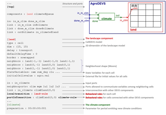
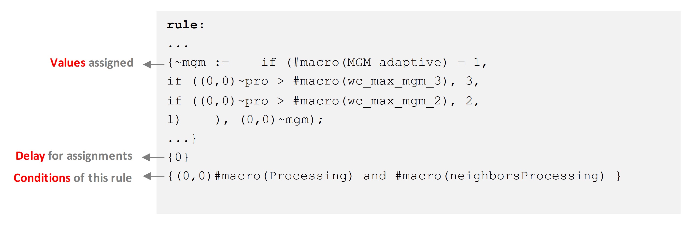
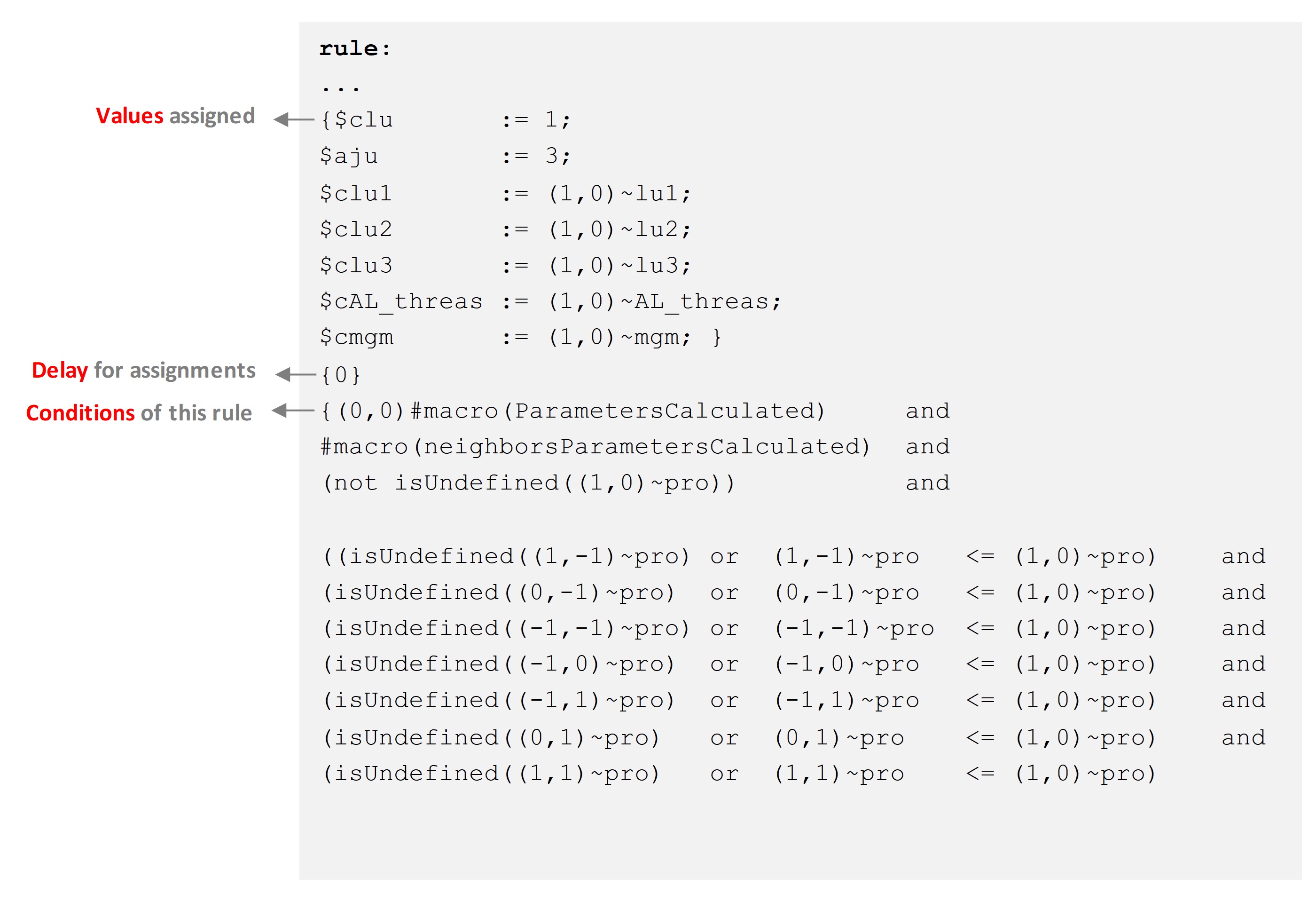
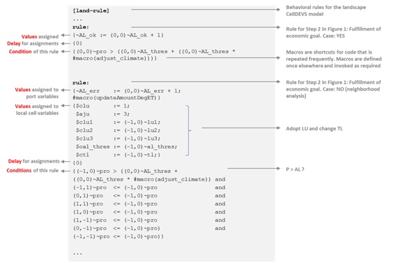
In Figure 19 we can see the main statements defining structure, components and interconnections through input-output ports. In Figure 20 we provide an excerpt of the agrodevs.ma file highlighting relevant lines. Note that three dots “…” in the figures denote lines omitted for the sake of brevity. In Figure 20 we can see main statements defining behavior for the landscape cellular automaton. Within each cell, a list of rules is evaluated sequentially in a top-down fashion, using a Value, Delay, Condition structure: the first rule that evaluates its Condition to true, will apply the Value to its attributes after a Delay amount of time. Once a rule is applied, the simulator recommences the cycle evaluating the rules from the top. This mechanism is applied asynchronously, simultaneously and in parallel to all cells in the model. The global timing for the whole cellular space is an emergent property driven by the local timing applied by each independent cell. The pairs \((X,Y)\) denote the positions for neighbors relative to each currently evaluated cell denoted with \((0,0)\).
Simulation framework and software experimentation environment
As discussed previously in the modelling approach section, AgroDEVS uses a DEVS-based formal approach. One salient feature of the DEVS formalism is the strict and clear separation between simulation algorithms and model specification. As a specialization of DEVS for Cellular Automata, the Cell-DEVS formalism inherits this separation. Different Cell-DEVS-capable simulators should be able to simulate a given Cell-DEVS model. In turn, different interactive user interfaces can be used to help with the design and maintenance of model specifications and to interact with the simulation exercises. Figure 21 shows a high-level component and deployment diagram of AgroDEVS.
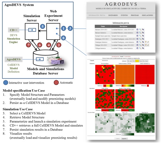
The CD++ generic simulation engine for DEVS and Cell-DEVS models resides in a Simulation Server. It can retrieve and simulate Cell-DEVS formal specifications of models that are stored in a Database Server. Such models can be written directly by specialists in the Cell-DEVS formalism or by higher-level experts in the agricultural domain using a friendly web-based interface. Once models are defined, they can be reused to launch as many simulation experiments as required, by invoking the simulator also from a web-based experiment interface. Figure 21 describes sequences of steps for two typical use cases: Model Specification and Simulation, denoting the components involved in each of them.
Appendix F. Design Concepts
Emergence
Four main landscape-level attributes emerge from individual farmer’s behavior and interactions among agents: (a) land use (% of cropping area under each crop type), (b) economic profit (the average landscape profit per hectare), (c) emergy renewability level (the average fraction of renewable emergy consumption in the landscape), and (d) the average rate of fulfillment of two thresholds: 1) a fixed environmental threshold, in terms of emergy renewability level (\(RL\)), and 2) a dynamic aspiration level, in terms of economic profit (\(P\)).
Adaptation
Agents can adjust their crop type allocation if the economic profit (at farm level) does not reach the \(AL\) at each \(CC\). In addition, each agent has two different adaptation mechanisms: a) adopting different \(TL\) based on the capital availability, and b) adjusting it’s \(AL\) based on both the \(WGC\) of each \(CC\) and the outcome in the previous \(CC\) (see sub-model section for computational details).
Objectives
Agents pursue to achieve a \(P\) level in each \(CC\) above their \(AL\) while satisfying (or not) a fixed \(RL\). If \(P\) is below agents’ \(AL\), they will be unsatisfied and will seek a different crop type allocation in the agents’ neighborhood. If an agent’s capital availability drops below the \(WCT\) for each \(TL\), they must adopt a lower-cost \(TL\), but agents never quit farming. Both landscape and individual \(RL\) emerge from the crop allocation decided for each agent, but it is not used as a farmer´s goal. Rather, this is an emergent property due to local rules.
Prediction
Agents predict the future consequences of their decisions (i.e., they build expectations) about \(P\) based on past outcomes and current weather information (\(WGC\)), following the theory of adaptive expectations (Shell & Stiglitz 1967). Agents revise their \(AL\) in each \(CC\) using adaptive rules based on a) the dissimilarity -in the previous \(CC\)- between the predicted and the observed \(P\), and b) the seasonal climate forecasts (\(WGC\)) for the current \(CC\) (see sub-model section for algorithms adjusting \(AL\)).
Sensing
Agents have information about their capital availability and consider this variable in their decisions about the potential adoption of higher (or lower) \(TL\). In addition, they are aware of the \(P\) achieved by their eight neighbors (Moore neighborhood) during each \(CC\). Finally, farmers are informed about the expected status of external contextual factors (i.e. seasonal forecast) for the current \(CC\).
Agent–Agent interaction
Agent interaction is based on the imitation of the crop type allocation of the best neighboring agent (i.e., the highest \(P\) achieved in the neighborhood) in the case of dissatisfaction with its own \(P\) achieved (as compared to its \(AL\)). Otherwise, the agent repeats its current crop type allocation in the next \(CC\).
Agent–environment interaction
Crop yield simulations reflect the interaction between farm decisions and both climate and soil conditions. These models capture the \(TL\) effect (through increasing fertilization and pesticide use) as well as the \(WGC\) of each \(CC\) (mainly global radiation and precipitation) and land quality factors (which are constant during the simulation). As crop simulation models represent biotic-unconstrained yield potential, final yields are adjusted in each combination of crop type-\(TL\) using potential weeds and pest infestation losses (see simulations input section for an example of crop yield data). Agent decisions have no effect on resource dynamics, through crop type allocation, and it is only on the current \(WGC\) that agents receive feedback about changes in resource conditions.
Stochasticity
Stochasticity is used to assign the \(TL\) and the crop type allocation to each agent only at the initialization procedure.
Collectives
Agents do not form or belong to aggregations that affect or are affected by other agents in the model version described here. Further model refinements should include collectives.
Appendix G. Acronym Table
| Acronym | Full form | Units |
|---|---|---|
| ABM | Agent-Based Model | |
| AL | Aspiration level | US$/ha |
| CA | Cellular Automata | |
| CAL | Climate-adjusted Aspiration Level | US$/ha |
| CC | Cropping Cycle | |
| DEVS | Discrete Event Systems Specification | |
| ET | Environmental threshold | % |
| IOF | Index of Observed Fit | |
| LU | Land Use (also crop type allocation) | % |
| LUCC | Land-use and Cover Change | |
| M | Maize cropping | % |
| O/T | Owner/Tenant ratio | Ratio |
| ODD | Overview, Design concepts, and Details | |
| OPA | Ordinal Pattern Analysis | |
| P | Profit | US$/ha |
| PM | Probability of a match | |
| RL | Renewability level | % |
| RP | Rental Price | US$ |
| S | Soybean cropping | % |
| SA | Sensitivity Analysis | |
| TL | Technological level | |
| V | Normalized RMSE | |
| W/S | Wheat/Soybean double-cropping | % |
| WGC | Weather Growing Conditions | |
References
AACREA. (2014). Survey of the goals and decisions of agribusiness decision-makers. Asociación Argentina de Consorcios Regionales de Experimentación Agrícola (AACREA). Website: www.aacrea.org.ar.
AGOSTINHO, F., Ambrosio, L. A., & Ortega, E. (2010). Assessment of a large watershed in Brazil using emergy evaluation and geographical information system. Ecological Modelling, 221(8), 1209–1220.
AHRWEILER, P., & Gilbert, N. (2005). Caffè Nero: The evaluation of social simulation. Journal of Artificial Societies and Social Simulation, 8(4), 14: https://www.jasss.org/8/4/14.html.
BALMANN, A. (1997). Farm-based modelling of regional structural change: A cellular automata approach. European Review of Agricultural Economics, 24, 85–108.
BERGER, T. (2001). Agent‐based spatial models applied to agriculture: A simulation tool for technology diffusion, resource use changes and policy analysis. Agricultural Economics, 25(2–3), 245–260.
BERT, F. E., Podestá, G. P., Rovere, S. L., Menéndez, A. N., North, M., Tatara, E., Laciana, C. E., Weber, E., & Toranzo, F. R. (2011). An agent based model to simulate structural and land use changes in agricultural systems of the Argentine Pampas. Ecological Modelling, 222(19), 3486–3499.
BERT, F. E., Rovere, S. L., Macal, C. M., North, M. J., & Podestá, G. P. (2014). Lessons from a comprehensive validation of an agent based-model: The experience of the Pampas Model of Argentinean agricultural systems. Ecological Modelling, 222, 284–298.
BOLCER. (2015). Relevamiento de tecnología agrícola aplicada de la bolsa de cereales, Argentina. Available at: http://www.bolsadecereales.com/retaa.
BONABEAU, E. (2002). Agent-based modeling: Methods and techniques for simulating human systems. Proceedings of the National Academy of Sciences, 99(3), 7280–7287.
BROWN, C., BROWN, K., & Rounsevell, M. (2016). A philosophical case for process-based modelling of land use change. Modeling Earth Systems and Environment, 2(2), 1–12.
BROWN, M., Campbell, D., Comar, V., Huang, S., Rydberg, T., Tilley, D., & Ulgiati, S. (2001). Emergy synthesis: Theory and applications of the emergy methodology. Center for Environmental Policy, University of Florida, Gainesville.
CASTELLA, J. C., & Verburg, P. H. (2007). Combination of process-oriented and pattern-oriented models of land-use change in a mountain area of Vietnam. Ecological Modelling, 202(3–4), 410–420.
COOK, D. J. (2009). Multi-agent smart environments. Journal of Ambient Intelligence and Smart Environment, 1(1), 51–55.
COOLEY, P., & Solano, E. (2011). Agent-based model (ABM) validation considerations. Proceedings of the Third International Conference on Advances in System Simulation (SIMUL 2011).
DEWULF, J., Van Langenhove, H., & Van De Velde, B. (2005). Exergy-Based efficiency and renewability assessment of biofuel production. Environmental Science & Technology, 39(10), 3878–3882.
EDMONDS, B. (2017). 'Different modelling purposes.' In B. Edmonds & R. Meyer (Eds.), Simulating Social Complexity (pp. 39–58). Berlin Heidelberg: Springer.
EVANS, T. P., & Kelley, H. (2004). Multi-scale analysis of a household level agent-based model of landcover change. Journal of Environmental Management, 72(1–2), 57–72.
FERRARO, D. O., & Benzi, P. (2013). A long-term assessment of the emergy use in an Argentinean agroecosystem, 19th biennial ISEM Conference.
FERRARO, D. O., & Benzi, P. (2015). A long-term sustainability assessment of an Argentinian agricultural system based on emergy synthesis. Ecological Modelling, 306, 121–129.
FILIPPI, J. B., Komatsu, T., & Hill, D. R. (2010). 'Environmental models in DEVS: Different approaches for different applications.' In G. A. Wainer & P. J. Mosterman (Eds.), Discrete-Event Modeling and Simulation: Theory and Applications (p. 30). Boca Raton, FL: CRC Press.
GARCÍA, G. A., GARCÍA, P. E., Rovere, S. L., Bert, F. E., Schmidt, F., Menéndez, A. N., Nosetto, M. D., Verdin, A., Rajagopalan, B., Arora, P., & Podestá, G. P. (2019). A linked modelling framework to explore interactions among climate, soil water, and land use decisions in the Argentine Pampas. Environmental Modelling & Software, 111, 459–471.
GIANNETTI, B., Almeida, C., & Bonilla, S. (2010). Comparing emergy accounting with well-known sustainability metrics: The case of Southern Cone Common Market, Mercosur. Energy Policy, 38(7), 3518–3526.
GILBOA, I., & Schmeidler, D. (2001). A Theory of Case-Based Decisions. Cambridge: Cambridge University Press.
GOTTS, N. M., & Polhill, J. G. (2009). When and how to imitate your neighbours: Lessons from and for FEARLUS. Journal of Artificial Societies and Social Simulation, 12(3), 2: https://www.jasss.org/12/3/2.html.
GRIMM, V., Berger, U., De Angelis, D. L., Polhill, J. G., Giske, J., & Railsback, S. F. (2010). The ODD protocol: A review and first update. Ecological Modelling, 221(23), 2760–2768.
GROENEVELD, J., Müller, B., Buchmann, C. M., Dressler, G., Guo, C., Hase, N., Hoffmann, F., John, F., Klassert, C., Lauf, T., Liebelt, V., Nolzen, H., Pannicke, N., Schulze, J., Weise, H., & Schwarz, N. (2017). Theoretical foundations of human decision-making in agent-based land use models – A review. Environmental Modelling & Software, 87, 39–48.
GRÖNLUND, E., Fröling, M., & Carlman, I. (2015). Donor values in emergy assessment of ecosystem services. Ecological Modelling, 306, 101–105.
HALL, A., Rebella, C., Ghersa, C., & Culot, P. (1992). 'Field-Crop systems of the Pampas.' In C. J. Pearson (Ed.), Ecosystems of the World (pp. 413–449). Amsterdam, NL: Elsevier.
HAPPE, K., Balmann, A., & Kellermann, K. (2004). The Agricultural Policy Simulator (Agripolis). An Agent-Based Model To Study Structural Change In Agriculture. Version 1.0 No. 918-2016-72618.
HAPPE, K., Balmann, A., Kellermann, K., & Sahrbacher, C. (2008). Does structure matter? The impact of switching the agricultural policy regime on farm structures. Journal of Economic Behavior & Organization, 67(2), 431–444.
HAPPE, K., Kellermann, K., & Balmann, A. (2006). Agent-based analysis of agricultural policies: An illustration of the agricultural policy simulator AgriPoliS, its adaptation and behavior. Ecology and Society, 11(1).
HARE, M., & Deadman, P. (2004). Further towards a taxonomy of agent-based simulation models in environmental management. Mathematics and Computers in Simulation, 64(1), 25–40.
INDEC. (1991). Censos nacional agropecuario 1988. Instituto Nacional de Estadística y Censos de la República Argentinas. A: Buenos Aires. Argentina
JONES, J. W., Hoogenboom, G., Porter, C. H., Boote, K. J., Batchelor, W. D., Hunt, L. A., Wilkens, P. W., Singh, U., Gijsman, A. J., & Ritchie, J. T. (2003). The DSSAT cropping system model. European Journal of Agronomy, 18(3–4), 235–265.
KAZI, B. U., & Wainer, G. (2018). Integrated cellular framework for modeling ecosystems: Theory and applications. Simulation, 94(3), 213–233.
KREMMYDAS, D., Athanasiadis, I. N., & Rozakis, S. (2018). A review of agent based modeling for agricultural policy evaluation. Agricultural Systems, 164, 95–106.
KÜPPERS, G., & Lenhard, J. (2005). Validation of simulation: Patterns in the social and natural sciences. Journal of Artificial Societies and Social Simulation, 8(4), 3.
LAMBIN, E. F., Turner, B. L., Geist, H. J., Agbola, S. B., Angelsen, A., Bruce, J. W., Coomes, O. T., Dirzo, R., Fischer, G., Folke, C., George, P. S., Homewood, K., Imbernon, J., Leemans, R., Li, X., Moran, E. F., Mortimore, M., Ramakrishnan, P. S., Richards, J. F., … Xu, J. (2001). The causes of land-use and land-cover change: Moving beyond the myths. Global Environmental Change, 11(4), 261–269.
LE, Q. B., Seidl, R., & Scholz, R. W. (2012). Feedback loops and types of adaptation in the modelling of land-use decisions in an agent-based simulation. Environmental Modelling & Software, 27–28, 83–96.
LEE, C. L., Huang, S. L., & Chan, S. L. (2008). Biophysical and system approaches for simulating land-use change. Landscape and Urban Planning, 86(2), 187–203.
LEE, S., Hong, J. H., Bae, J. W., & Moon, I. C. (2015). Impact of population relocation to city commerce: Micro-level estimation with validated agent-based model. Journal of Artificial Societies and Social Simulation, 18(2), 5: https://www.jasss.org/18/2/5.html.
LIGMANN-ZIELINSKA, A., Siebers, P. O., Magliocca, N., Parker, D. C., Grimm, V., Du, J., Cenek, M., Radchuk, V., Arbab, N. N., & Li, S. (2020). “One Size Does Not Fit All”: A roadmap of purpose-Driven mixed-Method pathways for sensitivity analysis of agent-Based models. Journal of Artificial Societies and Social Simulation, 23(1), 6: https://www.jasss.org/23/1/6.html.
LIGTENBERG, A., van Lammeren, R. J. A., Bregt, A. K., & Beulens, A. J. M. (2010). Validation of an agent-based model for spatial planning: A role-playing approach. Computers, Environment and Urban Systems, 34(5), 424–434.
MANUEL-NAVARRETE, D., Gallopín, G., Blanco, M., Díaz-Zorita, M., Ferraro, D. O., Herzer, H., Laterra, P., Murmis, M., Podestá, G., Rabinovich, J., Satorre, E., Torres, F., & Viglizzo, E. (2009). Multi-causal and integrated assessment of sustainability: The case of agriculturization in the Argentine Pampas. Environment, Development and Sustainability, 11, 612–638.
MARGENES Agropecuarios. (2015). Estadisticas agrícolas. Margenes Agropecuarios: Buenos Aires, Argentina.
MELLINO, S., Buonocore, E., & Ulgiati, S. (2015). The worth of land use: A GIS–emergy evaluation of natural and human-made capital. Science of the Total Environment, 506–507, 137–148.
MERCAU, J. L., Dardanelli, J. L., Collino, D. J., Andriani, J. M., Irigoyen, A., & Satorre, E. H. (2007). Predicting on-farm soybean yields in the pampas using CROPGRO-soybean. Field Crops Research, 100(2), 200–209.
MERCAU, J., Satorre, E. H., Otegui, M. E., Maddoni, G. A., Cárcova, J., Ruiz, R., Uribelarrea, M., & Menendez, F. (2001). Evaluación a campo del comportamiento del modelo CERES en cultivos de maíz del norte de la provincia de Buenos Aires. VII Congreso Nacional de Maíz. AIANBA. Pergamino, Buenos Aires, Argentina.
MOSCATELLI, G., Salazar Lea Plaza, J. C., Godagnogne, R., Gringberg, H., Sánchez, J., Ferrao, R., & Cuenca, M. (1980). Mapa de suelos de la provincia de Buenos Aires 1:500000. Actas de la IX Reunión Argentina de la Ciencia del Suelo. Asociación Argentina de la Ciencia del Suelo.
MOSS, S. (2008). Alternative approaches to the empirical validation of agent-based models. Journal of Artificial Societies and Social Simulation, 11(1), 5: https://www.jasss.org/11/1/5.html.
MÜLLER, B., Bohn, F., Dreßler, G., Groeneveld, J., Klassert, C., Martin, R., Schlüter, M., Schulze, J., Weise, H., & Schwarz, N. (2013). Describing human decisions in agent-based models – ODD + D, an extension of the ODD protocol. Environmental Modelling & Software, 48, 37–48.
NGUYEN, T. G., & de Kok, J. L. (2007). Systematic testing of an integrated systems model for coastal zone management using sensitivity and uncertainty analyses. Environmental Modelling & Software, 22(11), 1572–1587.
ODUM, H. T. (1996). Environmental Accounting: Emergy and Environmental Decision Making. Hoboken, NJ: John Wiley; Sons.
PARUELO, J. M., Guerschman, J. P., & Verón, S. R. (2005). Expansión agrícola y cambios en el uso del suelo. Available at: https://www.agro.uba.ar/.
PENGUE, W. A. (2009). Cuestiones económico-ambientales de las transformaciones agrícolas enCuestiones económico-ambientales de las transformaciones agrícolas en las Pampas. Problemas Del Desarrollo, 40(157), 137–161.
POLHILL, J. G., Sutherland, L. A., & Gotts, N. M. (2010). Using qualitative evidence to enhance an agent-based modelling system for studying land use change. Journal of Artificial Societies and Social Simulation, 13(2), 10: https://www.jasss.org/13/2/10.html.
PORTO, A., & Lodola, A. (2013). Economic policy and electoral outcomes. Journal of Applied Economics, 16(2), 333–356.
RAILSBACK, S. F., & Grimm, V. (2011). Agent-Based and Individual-Based Modeling: A Practical Introduction. Princeton, NJ: Princeton University Press.
RAILSBACK, S., & Grimm, V. (2015). 'Sensitivity, uncertainty, and robustness analysis.' In S. Railsback & V. Grimm (Eds.), Agent-Based and Individual-Based Modeling: A Practical Introduction (pp. 291–307). Princeton, NJ: Princeton University Press.
SAGPYA. (2009). Estimaciones agrícolas de cereales, oleaginosas, algodón, maní y poroto. Ministerio de Agricultura, Ganadería y Pesca de la Nación Argentina. Available at: http://www.siia.gov.ar/index.php/series-por-tema/agricultura. Last Access: July 2012.
SATORRE, E., Menéndez, F., Tinghitella, G., & Cavasassi, J. (2005). Triguero: Un sistema de apoyo a la fertilización nitrogenada de trigo. Convenio AACREA y PROFERTIL SA. Software de aplicación agronómico.
SCHREINEMACHERS, P., & Berger, T. (2011). An agent-based simulation model of human–environment interactions in agricultural systems. Environmental Modelling & Software, 26(7), 845–859.
SCHREINEMACHERS, P., Berger, T., & Aune, J. B. (2007). Simulating soil fertility and poverty dynamics in Uganda: A bio-economic multi-agent systems approach. Ecological Economics, 64(2), 387–401.
SHANMUGANATHAN, S., Sallis, P., & Buckeridge, J. (2006). Self-organising map methods in integrated modelling of environmental and economic systems. Environmental Modelling & Software, 21(9), 1247–1256.
SHELL, K., & Stiglitz, J. E. (1967). The allocation of investment in a dynamic economy. The Quarterly Journal of Economics, 81(4), 592–609.
SORIANO, A., León, R. J. C., Sala, O. E., Lavado, R. S., Deregibus, V. A., Cahuépé, M. A., Scaglia, O. A., Velázquez, C. A., & Lemcoff, J. H. (1991). 'Río de la Plata grasslands.' In R. T. Coupland (Ed.), Ecosystems of the World 8A. Natural Grasslands. Introduction and Western Hemisphere (pp. 367–407). Amsterdam, NL: Elsevier.
SOULE, M. J., Tegene, A., & Wiebe, K. D. (2000). Land tenure and the adoption of conservation practices. American Journal of Agricultural Economics, 82(4), 993–1005.
STERN, T. A. (2003). System and method for automated annotation of files. Google Patents.
THORNGATE, W., & Edmonds, B. (2013). Measuring simulation-observation fit: An introduction to ordinal pattern analysis. Journal of Artificial Societies and Social Simulation, 16(2), 4.
TITTONELL, P. (2014). Ecological intensification of agriculture — Sustainable by nature. Current Opinion in Environmental Sustainability, 8, 53–61.
TROITZSCH, K. G. (2004). Validating simulation models. Networked Simulations and Simulation Networks. Pages 265-270.
VAN Ittersum, M. K., & Rabbinge, R. (1997). Concepts in production ecology for analysis and quantification of agricultural input-output combinations. Field Crops Research, 52(3), 197–208.
VELDKAMP, A., & Verburg, P. H. (2004). Modelling land use change and environmental impact. Journal of Environmental Management, 72(1–2), 1–3.
VERBURG, P. H., de Nijs, T. C. M., Ritsema van Eck, J., Visser, H., & de Jong, K. (2004). A method to analyse neighbourhood characteristics of land use patterns. Computers, Environment and Urban Systems, 28(6), 667–690.
VERBURG, P. H., Schot, P. P., Dijst, M. J., & Veldkamp, A. (2004). Land use change modelling: Current practice and research priorities. GeoJournal, 61(4), 309–324.
VIGLIZZO, E. F., Pordomingo, A. J., Castro, M. G., LÉrtora, F. A., & Bernardos, J. N. (2004). Scale-dependent controls on ecological functions in agroecosystems of Argentina. Agriculture, Ecosystems and Environment, 101(2004), 39–51.
WAINER, G. (2006). Applying Cell-DEVS methodology for modeling the environment. Simulation, 82(10), 635–660.
WILENSKY, U., & Rand, W. (2007). Making models match: Replicating an agent-based model. Journal of Artificial Societies and Social Simulation, 10(4), 2: https://www.jasss.org/10/4/2.html.
YUN, T. S., & Moon, I. C. (2020). Housing market agent-Based simulation with loan-To-Value and debt-To-Income. Journal of Artificial Societies and Social Simulation, 23(4), 5: https://www.jasss.org/23/4/5.html.
YUN, W. S., Moon, I. C., & Lee, T. E. (2015). Agent-based simulation of time to decide: Military commands and time delays. Journal of Artificial Societies and Social Simulation, 18(4), 10: https://www.jasss.org/18/4/10.html.
ZAPATERO, M., Castro, R., Wainer, G., & Hussein, M. (2011). Architecture for integrated modeling, simulation and visualization of environmental systems using GIS and Cell-DEVS. Simulation Conference: Phoenix, AZ, USA.
ZEIGLER, B. P., Praehofer, H., & Kim, T. G. (2000). Theory of Modeling and Simulation: Integrating Discrete Event and Continuous Complex Dynamic Systems. Cambridge, MA: Academic Press.
ZEIGLER, B., Sarjoughian, H. S., Duboz, R., & Soulie, J. C. (2012). Guide to Modeling and Simulation of Systems of Systems. Berlin Heidelberg: Springer Science & Business Media.