Generation of Synthetic Populations in Social Simulations: A Review of Methods and Practices

,
and
aIRD, France; bINRAE, France; cIRD Vietnam
Journal of Artificial
Societies and Social Simulation 25 (2) 6
<https://www.jasss.org/25/2/6.html>
DOI: 10.18564/jasss.4762
Received: 07-Aug-2021 Accepted: 03-Mar-2022 Published: 31-Mar-2022
Abstract
With the aim of building realistic model of social systems, designers of agent-based models tend to incorporate more and more data and this data is of course having an impact on their outcomes. Among these data, those concerning the attributes of social agents, which together compose synthetic populations, are particularly important, but are usually difficult to collect and therefore to use in simulations. In this paper, we review the state of the art of methodologies and theories for building realistic synthetic populations for agent-based simulation models, as well as practices in the field of social simulation. We highlight, in particular, the discrepancies between theory and practice and outline the challenges in bridging this gap using a quantitative and narrative review of work published in JASSS between 2011 and 2021. Finally, we presents some ideas that can help modelers adopt better practices regarding synthetic population generation.Introduction
Agent-based simulations are widely used in the social sciences to study complex socio-environmental systems. Early models tended to be extremely simple and abstract, following the KISS approach (Axelrod 1997). However, there is a current trend which pertains to the development of richer data driven models following the KIDS approach (Edmonds & Moss 2005). This development is driven by the increased use of models as predictive tools in a decision support context. As in any agent-based model, agent behavior is considerably influenced by agent attributes, as observed for example, in the ABM on COVID-19, which establishes a strong correlation between the outcome of the disease and the structure of social contacts or age of agents (Hoertel et al. 2020). However, since these models must reflect realistic social dynamics, it is essential that agents’ attributes reflect real attributes of entities that they represent. This aspect is often achieved by generating a synthetic population of agents from the sociodemographic data available of the target population.
Schematically, a synthetic population is a simplified microscopic representation of the real target population: this population is a simplified record because it includes only a limited set of attributes of this target population – i.e., several attributes are not relevant considering the modeling objectives – and it is microscopic because all the entities and even sub-entities in the case of multilevel populations (e.g., individual in households) are explicitly represented as individual records (Guo & Bhat 2007; Ziemke et al. 2016). Because of this simplification and the need to vary scenarios, a synthetic population is never identical to the target population, but designed to match various aggregate statistical measures of the target population, such as the proportion of men and women or the age pyramid. In this context, the key challenge of synthetic population generation is to minimize any difference between generated and real populations in terms of the various indicators. This aspect however involves several problems: (a) data incompleteness: Data are often difficult to collect or do not fully represent the target population, and (b) data incongruity and inconsistency: When data can be collected, they are usually in different formats, with various encoding formats, at different scales and locations (c) once a population has been generated, it may be difficult to identify the appropriate indicators to measure any correspondences between the synthetic and target populations.
This article has two main contributions to facilitate synthetic population generation in social simulations. First, we have reviewed existing theories and methods used to generate a synthetic population in a social simulation model. Second, we have investigated the actual usage of these methods in the field. Specifically, we examined several hypotheses by conducting a systematic review of models published in the last ten years in JASSS:
- H-1 Despite increasing calls to base models on empirical data (Chattoe-Brown 2014; Edmonds & Moss 2005; Flache et al. 2017), only a small fraction of simulation models actually base agent population generation on intentional, well-designed methodologies.
- H-1a Initialization of agent attributes does not often use input data.
- H-1b Agent attribute values are often generated using generic purpose distributions.
- H-2 Descriptive models often rely on synthetic population generation methodologies.
The remaining article is structured as follows: Section 2 presents the methodological and theoretical background of synthetic population generation. Section 3 presents the review of related practices in the field of agent-based social simulation. In Section 4 and 5, we have given several recommendations that can help improve synthetic population generation practices.
Methods to Generate Synthetic Populations
This section introduces the field of synthetic population generation and lists the main methods that have been proposed thus far. For each proposed algorithm, we specify the required input data and expected generated results. First, we introduce the scope of this work and clarify several concepts of synthetic population generation.
Context
We would like to clarify what this review is not: This study focuses on only the generation of entities and their attributes, and does not consider the spatialization of those entities or generation of the social networks that connect them. Readers interested in the latter can refer to Chapuis et al. (2018) for the localization of synthetic agents and Amblard et al. (2015) for synthetic networks. Second, although synthetic population generation is not theoretically limited to the generation of human populations, we have limited the scope of this study to synthetic populations used in social simulation, which primarily encompasses populations of individuals and households.
Several critical reviews on the subject have been presented (Huang & Williamson 2001; Ryan et al. 2009). this review is an updated account of the work performed since then, focusing on the use of synthetic populations in the field of agent-based social simulation. Many of existing procedures and methods for generating synthetic populations (e.g., Felbermair et al. 2020 for synthetic population generation within MATSim, Hafezi & Habib 2014 for transportation microsimulation or Moeckel et al. 2003 for an influential TRANSIMS-related paper) pertain to a related but distinct field, i.e., transportation modeling, where ABM is one of the methodologies used among discrete event simulation, microsimulation and other equation-based modeling approaches. While this distinction does not affect the generality of the proposed procedures, it may influence the choice of tools and outcome expectations.
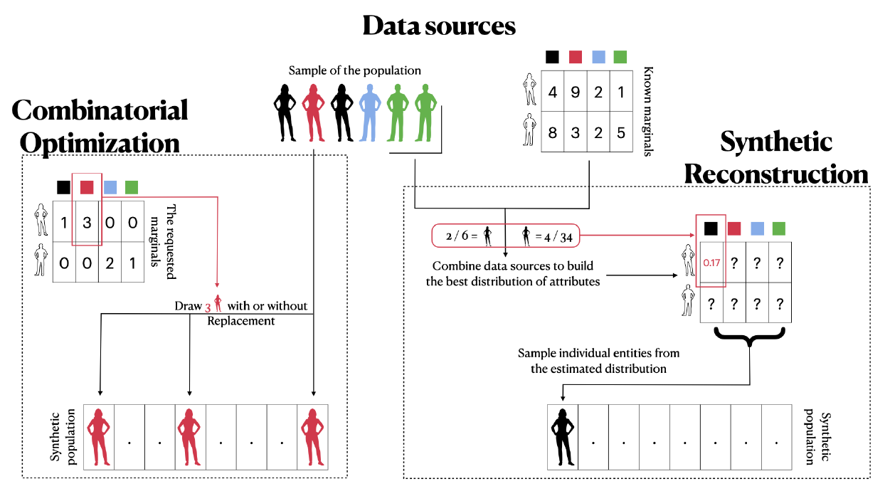
One principle that has been used to classify synthetic population methods is the type of input data, as this aspect is a crucial practical starting point: When modelers select an appropriate method to generate a synthetic population, they often make the decision based on available data. However, we consider it wise not to follow the classical, mostly theoretical, view that divides the field according to data requirements, i.e., sample-based vs. sample-free methods (e.g., Lenormand & Deffuant 2013; Ye et al. 2017). Several algorithms can be relevant with or without a sample, such as Bayesian-based generation (Sun & Erath 2015), while classical algorithms, such as the iterative proportional fitting (IPF) procedure (see Subsection 2.8), do not need to be used in the generation process. Therefore, instead of the input data type, we set the distinguishing criterion as the synthesis technique to either create the properties of the entities or reproduce known real entities, termed as synthetic reconstruction (SR) and combinatorial optimization (CO), respectively.
The first approach is based on the idea of synthetic reconstruction (Wilson & Pownall 1976) and consists of building populations through the random generation of individual characteristics. This process is usually conducted by drawing attribute values either from the available distributions (Barthelemy & Toint 2012; Gargiulo et al. 2010) or from an estimated joint distribution based on techniques such as the IPF algorithm (Stephan 1942) or the Markov chain Monte Carlo techniques (Casati et al. 2015). When individual profiles are available, the generation can be a replication of the individual profiles to fit the macroscopic descriptors available. This approach refers to Combinatorial Optimization (Williamson et al. 1998). Although it is less popular, several promising techniques have recently been established (Harland et al. 2012; Ma & Srinivasan 2015). Figure 1 summarizes the key ideas behind each procedure: As shown in the left part of the figure, the CO approach ultimately reproduces real records of individuals to fit a desired global statistical state of the synthetic population. In contrast, as shown in the right part of the figure, the SR approach is centered around extrapolation techniques to build the most relevant underlying distribution to draw synthetic entities from.
The two techniques are paradigmatic, meaning that they define the principles of an approach to build a synthetic population rather than a procedure that may be applied to generate it. Therefore, most of the reviewed procedures in this section deviate from the basic principles of CO and SR. For instance, SR techniques can be used to enhance the results of the CO algorithm to add new information to an existing synthetic population (Thiriot & Sevenet 2020) or use CO techniques to mix SR-based synthetic populations at several scales (Huynh et al. 2016; Watthanasutthi & Muangsin 2016). In addition to combining these approaches, many models build on the concepts of one technique, for instance, by using weights attached to individual records of microdata to build the targeted marginal objective in the CO perspective, known as re-weighting of the population sample (Tanton et al. 2014; Yameogo et al. 2021), or by using statistical learning techniques, such as copula functions (Jeong et al. 2016) or hierarchical mixtures (Sun et al. 2018) to build the underlying distribution of attributes in the SR perspective. In both cases, the procedure follows the concept of CO and SR approaches, i.e., to replicate known individual entities from a sample of real records and draw characteristics of the synthetic entities from an estimated distribution of attributes, respectively.
In the following subsections, we have presented a panorama of studies of synthetic population generation for use in agent-based modeling. Our perspective first explores the available data before the generation process: We first review typical data that can be used to generate a synthetic population. We then describe the main algorithms and techniques to generate a synthetic population from these inputs, mainly focusing on the SR and CO archetypal methodologies. Finally, we conclude the section by discussing how researchers assess the quality of the generated synthetic population.
First step: Working with data
To realize synthetic population generation, researchers usually adopt two types of data. First, macrolevel data, which consist of distributions (income distribution, age structure, etc.) or aggregated values (average age, quantiles of revenue, etc.); and second, data that consist of a set of individual records at the microlevel that represents a portion of the whole population.
Macrodata descriptors
The first type of data may be available as a contingency or frequency matrix known as a distribution of attributes. For example, a cell of the distribution matrix could be the number or proportion of male laborers aged between 16 and 24. The matrix is usually presented as table data in which the columns and rows describe attributes such as the age and gender, specified using categorical values, e.g., under 5 years old or male/female, respectively. The data table may have an unlimited number of dimensions and reflects the joint multiway distribution/contingencies of attributes. However, the data are often scattered, that is, one may access several tables, each displaying few attribute relationships. Because of the data heterogeneity associated with populations, the table often has missing values, usually in the form of unrecorded relationships between attributes (attributes that are not present in every data table). In certain cases, the data content may be relative to a specific attribute, especially in terms of the spatial distribution, for example, the proportion of males and females per ward. In this case, the frequency cannot be generalized and must be used according to the reference attribute distribution. A related issue arises when the attribute has a divergent encoding form across scattered data tables: for example, one matrix that crosses age encoded by range of 5 years with gender, and another matrix in which the age is encoded by custom ranges, as is usually the case when crossed with the occupation status; in this case, the age usually start at the legal age to work and is grouped into carrier dependent age ranges (e.g., 16-24, 25-35 or above 65).
Another type of macro data is the statistical aggregated data, such as the average, median or quantile value of an attribute. These data concern a single numerical attribute, such as the age, salary or size of the households. Such data are classically ignored in synthetic population generation but have been employed in recent methods (Gallagher et al. 2018; Saadi et al. 2016).
Most national statistical institutes release such data with open access. The data are often updated each year and reflect many social dimensions, such as work, consumption or opinion, in addition to basic demographic attributes.
Microdata descriptors
The second type of data represents a limited sample of the whole population: The data can be composed of individual records of 1%, 2%, 5%, and in rare cases, 10% or more of the population. Because microdata directly depict real individual characteristics, they are often limited in scope due to practical and ethical considerations, either by the number of individual records or number of characteristics per individual, and in most cases, on both points. In certain cases, the records represent a class of entities rather than a particular individual and are assigned weights that represent the degree of importance of this class of entities in the sample, i.e., entities with the same vector of attribute values, considering the limited scope of represented attributes.
Samples or microdata are often presented as table-based data, in which each row represents an individual entity, and each column represents an attribute for which the entity has a particular value. As mentioned before, when rows do not refer to individual entities but a class of entity, a column is dedicated to the weights that the type of entity represents in the overall sample.
Just like macro-data descriptors, the microdata of a population can usually be accessed through national statistical institutes on demand. A notable initiative led by the Integrated Public Use Microdata Series (IPUMS) makes it possible to freely access (requires identification) country-level sample data for approximately 100 countries worldwide.
Remarks on the data processing step in synthetic population generation
Most of available tools to generate synthetic populations have loose or heavily constrained ways to define the required input data. For instance, the iterative proportional updating (IPU) procedure proposed in Ye et al. (2017) must be fed with Public Use Microdata Series data (or PUMS, i.e., a sample of individual records with household identifiers, specified by the US census bureau), whereas the SPEW library (Gallagher et al. 2018) requires IPUMS microdata. In other words, even if modelers do have microdata, these must be formated in the style of the US-based census micro-data. Generalizing the principle means that for each synthetic population generation procedure, it is necessary to preprocess the data and adapt it to a specific data format. In this context, the existing synthetic population algorithms opt for one of two perspectives: focus on loosely defined types of data or manage a unique source of data. For the former approach, a considerable amount of effort is necessary to adapt data to the processing pipeline. The latter approach forces people to rely on a certain data format, leading to data manipulation to fit the required format and type, which is not always possible. Even if no processing pipeline can handle every data format, engaging in the generation of a synthetic population will always require data preprocessing to address several limitations.
In this section, we have summarized the major issues encountered by modelers interesting in building a synthetic population based on available loosely structured data.
Data incompleteness: The first issue relates to the missing parts in the data. This aspect is critical because it represents the principle of population synthesis: having a complete view of the entities’ attributes ensures the generation of the best possible synthetic population by simply reading the source data. In this regard, having access to a sample of the targeted population is often a simple and effective technique to build a synthetic population, which requires simply initializing agents as the exact reflections of individual records. When modelers want to adapt these microdata to particular constraints (e.g., specified spatial extensions, creation of more individuals than those in the data, or use of statistical weights attached to records), to add unrecorded attributes or when there is no sample available, missing data must be identified. In most cases, the lack of data is expressed by unrecorded relationships between attributes, and synthetic reconstruction attempts to combine multiple sources to compensate for this lack of information.
Data incongruity: When several pieces of information target the same attribute but with various encoding forms, there exists a mismatch between data records. For example, age can be encoded in various forms from continuous integer to categorical values of various ranges, and each range can be used differently when crossed with other attributes. For example, in the data provided by the French Institute of Statistics (INSEE), the age category begins at 16 and ends at 74 when crossed with professional status, whereas it is usually expressed as an integer when crossed with gender.
Data inconsistency: Available data can be present in various shapes, formats and contents. Except in the scenario in which modelers can base the generation process on a single source, data are usually scattered into pieces of information that first require harmonization to be used in conjunction for the population synthesis process. Generic tools to generate synthetic population, e.g., those proposed by Gallagher et al. (2018) and Chapuis et al. (2018), emphasis this harmonization step. In contrast, most influential theoretically proposed approaches in this domain minimize or simply ignore this aspect (Müller & Axhausen 2011; Sun et al. 2018; Ye et al. 2016). In particular, the approaches are based on a given and controlled set of data, and thus, the procedure may not be effective when slightly different data are input. This aspect is a key concern for the usability of the proposed methods in generating synthetic populations.
Second step: Generation of a synthetic population
In this sub-section, we describe the main procedures for generating synthetic populations in agent-based social simulations. The section involves two subsections: The first sub-section focuses on techniques similar to SR principles, in which the generation process is based on the estimation of the best possible underlying distribution of attributes; the second subsection is centered on techniques related to CO principles, in which the generation process is based on the available individual records of real entities to reproduce in the synthetic population.
Synthetic Reconstruction (SR)
SR defines a set of methods that reconstruct individual entities. From the perspective of SR generation, synthetic individuals are attribute vectors and the generation process consists of fulfilling each individual vector with appropriate values. We detail this generation procedure known as sampling in the following sub-section. In the next sub-section, we discuss distribution estimation algorithms that can be used to facilitate the sampling procedure.
Sampling procedure: Sampling methods include all methods based on the drawing of records associated with given distributions of probabilities. When applied to synthetic population generation, sampling is performed to determine the characteristics of individuals using discrete distribution of probabilities. In only very few cases, continuous distribution can be used. Sampling can be performed by selecting an entire vector of characteristics, e.g., an individual, or by gathering separately drawn characteristics.
The most basic sampling technique is the Monte Carlo method (Harland et al. 2012) that uses raw input data knowledge regarding the distribution of attributes. This default technique can be labeled direct sampling (DS) to emphasis that it relies on the raw available data. Individual characteristics can either be drawn sequentially or several at a time if the input data include records on relationships between attributes. However, with the increase in the number of population attributes, multiway joint distribution becomes infeasible. Therefore, a realistic dependency structure between attributes must be determined upstream. Subsequently, the synthetic population can be generated iteratively using Bayesian rules on conditional distributions (Gargiulo et al. 2010). Hierarchical sampling (HS) (Barthelemy & Toint 2012) is the most basic model to account for this type of sampling method. This solution is extremely flexible, but the user must manually define the hierarchy of attributes: which attribute(s) should be drawn first, followed by the other attributes to be drawn given the previously determined attribute value(s), to the last attribute.
The use of a Bayesian Network (BN) in synthetic population generation extends and generalizes the principle of HS by using a graphical model (Sun & Erath 2015). BN-based samplers work iteratively, drawing characteristics starting from the root node(s) and continuing down the network path of the graphical model. Such samplers have a notable advantage compared to HS as they can manipulate classical learning techniques to automatically determine the graphical model and/or missing parameters (see Paragraph 2.30). This approach is very flexible in terms of input data: it is relatively easy to learn parameters of the BN from macro and/or microdata (Thiriot & Kant 2008). The graphical model can be retrieved from the distribution of attributes when they are available but must be estimated when initialized using microdata (Sun & Erath 2015).
Recently, several contributions (Casati et al. 2015; Farooq et al. 2013; Saadi et al. 2016) have launched a new trend in SR, based on the use of Markov Chain Monte Carlo (MCMC) methods. The Gibbs sampling algorithm (Farooq et al. 2013) has been used to directly sample individuals using a simulated distribution through Markov chains. Combined with a fitting algorithm, this procedure can generate complex and reliable synthetic populations (Casati et al. 2015).
In addition, SR methodologies based on graphical model such as HS, BN and MCMC, are suitable in cases in which modelers need a multilayered synthetic population. In contrast to the basic Monte Carlo sampling methodologies, the graphical model can mix items – i.e., the nodes with attached parameters or states with transition state probabilities – to assess the attribute probability distribution of several types of entities. For example, Sun & Erath (2015) generated individuals into households using a unique graphical model to represent the distribution of attributes for both types of entities, while (Casati et al. 2015) generated the same type of synthetic population using a Markov Chain model to represent both individual and household entities.
Distribution estimation algorithm: These algorithms sample characteristics from known distribution(s) of attributes. A key drawback is that all unknown relationships between attributes are statistically independent in the generated synthetic population. Because a higher distribution quality corresponds to a superior sampled population, the estimation of the underlying multi-way joint distribution of attributes can enhance the sampling output. In the literature, this procedure is also referred to as the fitting step in SR methodologies. We would like to emphasize that this step is not mandatory, and many SR algorithms, such as DS or HS, do not use distribution estimation algorithms. Recently, algorithms such as the Gibbs sampling MCMC, which is a distribution estimation and sampling technique in one framework, have been adopted. Here, we have reviewed the most commonly used techniques to estimate the underlying multiway distribution.
The iterative proportional fitting (IPF) (Beckman et al. 1996) process is widely used in the domain of synthetic population generation (Müller & Axhausen 2010). The algorithm fits each cell of a \(n\)-dimensional matrix (distribution of attributes) according to known marginal controls (Stephan 1942). The algorithm uses sample data as a seed to fill the matrix that describes the distribution of attributes, and iteratively updates the matrix cells to fit the known contingency dimensions. For more details regarding the mathematical description and new insights, please refer to the work of (Lovelace et al. 2015).
IPF has been criticized in many aspects, including the “zero cell problem” (Choupani & Mamdoohi 2016), the “curse of dimensionality” (Casati et al. 2015) and potential non-convergence of the algorithm. The most notable issue, however, is the inability of considering multiple statistical levels of constraints – i.e., multi-layered populations (Guo & Bhat 2007). Hierarchical IPF (Müller & Axhausen 2011) and IPU (Ye et al. 2009) have been developed to overcome this issue. These methods compute the factors and weights associated with individual and household records either iteratively or by using household and individual categorization, respectively. The basic idea of proportional updating is the same as that of the original IPF procedure. The main difference pertains to the definition of the matrix dimension and marginals. These techniques have been developed in the narrow context of individuals in households and have only been used with a two-layered population. Moreover, these approaches necessitate preprocessing of the input data to fit the algorithm requirements and are extremely stringent regarding the type of data needed: sample and aggregated data must be available at both the individual and household levels.
Recently, MCMC (Farooq et al. 2013) and BN (Sun & Erath 2015) models have been used to represent the population distribution of attributes. Both framework provide the user with a graphical model and techniques to estimate the missing data. For example, the Metropolis-Hasting algorithm can estimate the multiway joint distribution through the MCMC procedure (Kim & Lee 2015), while several fitness-based learning algorithms can be used to estimate the BN graphical model and its parameters (Sun et al. 2018). These two methodologies can help establish sampling algorithms based on a Markov chain or Bayesian network and joint/conditional distribution estimation techniques that can be used for single-layered populations and multilayered populations.
Emerging deep learning trends: The last addition to the set of SR techniques are deep learning generative methods. The use of a deep neural network (DNN) is straightforward. A DNN refers to as a set of techniques to learn an extremely sophisticated network embedded version of the underlying distribution from a vector based representation of records in a data set. Here, the autoencoder approach is particularly effective for data synthesis. The concept of such DNNs is to train two networks. The first network decreases the dimensionality of the data to a bottleneck representation, while the second network expands this shortened representation to a fully explicit record. Using unsupervised learning techniques, these two adversarial networks can learn how to generate new records and have been used in the context of transport-related research, especially in the form of a variational autoencoder (VAE) (Garrido et al. 2020). However, the learning curve of such algorithms is a limitation. Although these algorithms are effective when provided with an extremely large set of data, their performance is inferior when there are few data records, there are missing data (i.e., data incompleteness) and they appear in various shapes and format (i.e., data incongruity and inconsistency), as is usually the case in population synthesis (see Subsection 2.8).
Combinatorial optimization (CO)
CO methods draw individuals from a sample, with or without replacement, to satisfy a fitness criterion. This convergence criterion is usually built using input data regarding the distribution of attributes at the macrolevel. In the following sub-section, we have briefly examined the fitness computation procedures and optimization algorithms used to monitor CO-based generation.
Fitness computation procedures: The objective of fitness computation is to assess the distance between the distribution of attributes in a generated population and information available regarding the real distribution of attributes. The fitness can be computed using two types of aggregations: Numerical aggregation, based on an aggregated account of distance, such as the standard root mean square error (SRMSE) (Otani et al. 2010); and categorical aggregation, based on a Hamming-like distance, for example the total absolute error (TAE), which is the sum of misclassified records in a synthetic population (Williamson et al. 1998). In most cases, the fitness indicator is similar to that used to evaluate the quality of the generated population (Subsection 2.38). Hence, the CO principle is to maximize the general quality of the generated synthetic population through an iterative optimization process. A custom fitness function could be used based on several indicators, such as the statistical moment on different attributes (e.g., quartile of income or mean age), combined with several well-known indicators such as SRMSE and TAE. In most cases, a single aggregated fitness criterion fulfills the requirement even if multi-criteria fitness function could be used. However, these functions are difficult to monitor and may considerably increase computation time. Finally, although fitness computation can be realized using only raw input data, CO methods generally rely on a distribution estimation algorithm such as IPF (Voas & Williamson 2000) to enhance the knowledge regarding the targeted distribution of attributes.
Optimized sampling algorithm: In principle, all fitness-based optimization algorithms can be used to generate a synthetic population from a CO perspective. Simulated annealing (Harland et al. 2012), hill climbing (Kurban et al. 2011), genetic algorithms (Said et al. 2002) and greedy heuristic (Srinivasan et al. 2008) approaches have been used in this context. The procedure involves the establishment of an initial random population from a sample and iterative modification of the initial solution to obtain a higher fitness (Williamson et al. 1998). The mechanism that changes the population depends on the algorithm and modeler’s choice. The most commonly used strategy is to swap a randomly selected individual with a potential replacement individual; however, the scope is not limited to this transition function. For example, in their hybrid solution to synthetic population generation, Barthelemy & Toint (2012) modified the individual’s characteristics to enhance the overall fitness. Globally, the crucial concept is to compute a close solution (often termed a neighbor) and move along a path of randomly selected solutions to find the most satisfying solution. No theoretical requirement is imposed on the movement of one solution to another, and several individuals can be swapped along with stringent selection criteria (for example, two individuals who have vectors of attributes with a given Hamming distance in their respective vectors of attributes can be swapped). In the optimization process, genetic algorithms have not been widely used but appear to be promising and flexible candidates (Williamson et al. 1998). These algorithms maintain multiple solutions and combine them iteratively to achieve a superior solution. Unlike simulated annealing, tabu search or hill climbing algorithms, genetic algorithms are less susceptible to be stuck in local optimal solutions (Otani et al. 2010). However, these algorithms involve a large number of parameters and require considerable modeling effort. Notably, the overall optimization procedure from the CO perspective depends considerably on the modelers’ choices regarding the fitness criteria and generation and exploration of neighbors’ solutions. These questions do not have default or basic answers and must be addressed by the modelers.
Last step: Validation of the synthetic population
Validation is usually performed considering the distance metric between generated and input marginals for the attributes of synthetic entities, e.g., distance between the distribution of age in synthetic population and input data regarding the distribution of age. In most cases, the quality of the synthetic population is assessed using the same dataset that has been used for the generation process. Hence, the validation of the synthetic population is performed out by measuring the distortion introduced by the generation process using the aforementioned distance metric. To this end, several indicators have been proposed.
Indicators: The total absolute error (TAE) is the simplest quality indicator. This error is the record of misclassified entities in the synthetic population (Williamson et al. 1998), with the misclassification evaluated using the absolute differences in the table or matrix cell. The TAE index examines the number of entities with particular attribute characteristics, such as being male or unemployed, and compares it to the number of people with these characteristics in the targeted population. When the relationships between the attributes are available, the indicator can examine the cross-classification, such as married males aged between 20 and 24 years. As an absolute indicator, TAE may be difficult to interpret. To alleviate this difficulty, the proportion of good prediction (PGP), which is the proportion of misclassified entities, can be used. In this case, the TAE is divided by the maximum absolute error that depends on the TAE computation and known relationship between attributes in the input data, i.e., the number of “classes” available in the input data and the number of classes compared to assess TAE.
In addition to the error for the overall population, the absolute average percentage difference (AAPD) or relative absolute error (RAE) can be considered to assess the average disruption introduced by the generation process. In contrast to PGP and TAE, these indicators focus on the expected error for any class of attribute (or combination of attributes) characteristics. Moreover, it would be interesting to examine the standard deviation to better understand how misclassification is distributed along the distribution of attributes. The (standard) root mean square error (RMSE or SRMSE) is the most commonly used indicator. This indicator is similar to the two preceding indicators as its core mechanics is to aggregate the error over each class of records in the input data. However, this value can be computed in several ways, rendering it complex to setup and understand in the context of synthetic population; see Zhu & Ferreira (2014), Müller & Axhausen (2011) and Otani et al. (2010) for three diverging definitions.
More promising but complex indicators include the relative sum of squared Z-score (RSSZ) (Huang & Williamson 2001) and RSSZ* (with a modified Z-score) (Williamson 2012). These indicators can aggregate both errors for the entire population and each class of records into a single indicator.
Table 1 presents an overview of the reported fitting measures used to assess the synthetic population quality. We have attempted to provide synthetic information regarding these measures: the type of difference that the measures encode (relative or absolute), the scale at which these measures operate (global or local) and a synthetic mathematical notation. It is difficult to specify a unique notation to describe how each measure is computed, mostly because different authors use their own notation and there is a lack of homogeneity in the definition of certain measures. For simplicity, we denote a vector of attribute values as \(x\), where \(X\) is the set of all possible vectors, \(T_x\) (\(T'_x\)) is the actual number (proportion) of known real entities with vector \(x\) and \(E_x\) (\(E'_x\)) is the estimated count (distribution).
| Name | Type | Scale | Formulation |
|---|---|---|---|
| TAE | Absolute | Global | \(\sum_x^X |T_x - E_x|\) |
| PGP | Absolute | Global | \(\frac{\sum_x^X T_x \equiv E_x}{|X|}\) |
| AAPD | Relative | Global | \(\sum_x^X |T_x - E_x| / T_x\) |
| SRMSE | Relative | Global | \(\frac{\sqrt{\sum_x^X (T_x - E_x)^2}}{\sum_x^X T_x}\) |
| RSSZ | Relative | Local | \(z_x = \frac{E'_x - T'_x}{\sqrt{T'_x (1 - T'_x)}/T_x}\) and \(RSSZ = \sum^X_x \frac{Z_x^2}{C_x}\) with \(C_x\) the \(5\% \chi^2\) for \(x \in X\) |
For an overview of indicators to assess the synthetic population goodness-of-fit, readers can refer to the related works focusing on that point, e.g., Voas & Williamson (2000) and Timmins & Edwards (2016).
Synthetic Population Generation in Social Simulations
As mentioned in the previous section, many methods have been established to build synthetic populations. As described in the following sections, we investigated how these methods are actually used by social simulation modelers. To answer this question, we analyzed published models and identified the methods used to generate the set of simulated agents.
In general, performing such analyses is time consuming because it requires the examination of the models regarding the initialization of agents and the code to identify the actual algorithm(s) used to generate agents’ attributes. Following a semisystematic literature review methodology, we focused on models published solely in JASSS. This method is semisystematic because it limits the search to resources published in a single journal, while relying on the systematic framework to filter and select relevant articles and extract and analyze the content of the models.
We reviewed papers published over ten years in JASSS as an indicator of the practices of social simulation modelers related to synthetic agent population generation. This review was limited to a single journal for two reasons: First, this journal is a key resource in the field of social simulation, and second, a canonical systematic search of thousands of publication titles yielded certain results on methodological aspects, but almost none on the actual initialization of social entities in simulation models. For instance, as of July 2021, a Google Scholar search with "synthetic population generation" returned mostly theoretical papers presenting a dedicated algorithm or approach to generate a synthetic population.1
Methodology
With the exception of the search phase, we chose to adhere to the requirements of systematic review and the PRISMA statements (Moher et al. 2009). These requirements included the selection of relevant articles based on a careful reading of the titles, abstract, and/or part of the article (selection phase in Screening Subsection); definition of a content extraction framework to build a coherent set of data from the relevant articles (content extraction phase in Extraction Subsection) and systematic analysis of the recorded content using a quantitative and narrative analysis review (analysis, synthesis and review phases in Section 3.11). Finally, we summarized the gaps and lessons learned from the practices to identify issues and challenges in using synthetic population generation in the field of agent-based social simulation.
Screening
The main criterion for selecting relevant papers for the analysis phase was simple: papers in JASSS that included a simulation model description were considered eligible. We excluded, a priori, all review papers and contributions that were not based on a simulation model, for example, a theoretical proposal such as that of Jager (2017). In several proposals, although a simulation model was included, the main focus was not the model itself but either the analysis of the simulation (e.g., Thiele et al. 2014), extensions of existing models (e.g., Taghikhah et al. 2021) or an application of a generic framework (e.g., Bourgais et al. 2020). Conversely, many papers presented theoretical models, which were not prima facie concerned with synthetic population generation due to the abstract nature of the simulated entities. Nevertheless, we chose to include these papers in the analysis to identify how modelers in this context choose to obtain the value of agents’ attributes and how this aspect relates to more refined synthetic population generation practices.
Moreover, we analyzed articles published between the 3rd issue of 2011 (June 2011) and the 2nd issue of 2021 (March 2021, the last available issue when this search was conducted). This range involved 478 articles spread over 40 issues, among which 342 featured a simulation model. Figure 2 presents the quantitative results of the eligibility step.
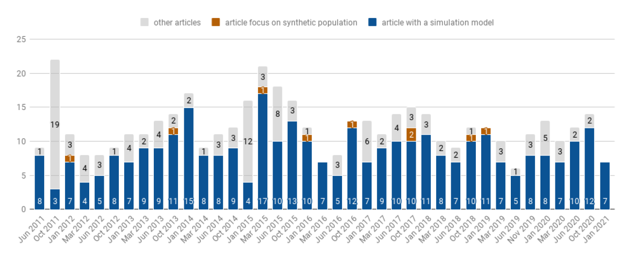
Despite the wide variety in the number of papers per issue, most issues were composed of a majority of papers describing a simulation model (between 3 and 17), with the exception of two special issues. Among the selected articles, 10 focus on the synthetic population, i.e., the main objective of the article is to present a method for generating a set of representative agents based on demographic data (Dumont et al. 2018; Harland et al. 2012; Huynh et al. 2016; Lenormand & Deffuant 2013; Lovelace et al. 2015; Smith et al. 2017; Wickramasinghe 2019; Yameogo et al. 2021; Ye et al. 2017, 2016).
Content extraction
In the systematic review exercise, content extraction referred to the extraction of data that served as the basis for a systematic content analysis. Explicit rules were used to format the content in a way that decreases the reader’s subjectivity.
The Hypothesis presented in the introduction guided the codebook used for content extraction. Specifically, we identified key aspects to answer questions regarding the procedure, input data, application scenario and adopted models. Content extraction was performed by first examining the eligibility in terms of the inclusion criteria, description of the model features and generation process.
- Following the PRISMA framework (Moher et al. 2009), the first step was to establish the eligibility criteria based on the title, abstract, and sequential reading of the article to assess inclusion or exclusion in the subsequent analysis step. If the article description contained a simulated model, the article was selected and we continued to extract the content; otherwise the article was excluded for further analysis.
- Once an article was considered for further analysis, we highlighted two main features of the model: first, the entities to be generated (i.e., agents) and their attributes, and second, information regarding the case study, including location, time, and whether GIS data were used. If the article involved a systematic protocol to describe the simulation model such as ODD or STESS, it was recorded, and most of the content extraction was based on parsing the protocol corresponding section, e.g., in the case of ODD, the entities, initialization, and input data sections (Grimm et al. 2010). Otherwise, we identified the corresponding sections in the article, and possibly examined the source code when possible.
- Finally, we examined the process of the agents’ generation. First, we identified whether an explicit process was presented in the article. We noted all the algorithms used to choose the value of the attributes, the algorithm parameters and the data types and sources that the algorithm is based on. The algorithm and data type were recorded using a closed list: constant, random function, calibration, synthetic reconstruction, combinatorial optimization, raw data, and NA for algorithm, and Sample, contingency, distribution, expert knowledge, statistical moment, and NA for data type.2 Readers can refer to Appendix A for more details on these categories.
All the information was recorded on a record sheet in a tabular format. Each criterion extracted from the reviewed articles and their related resources answered a given question, and the set of questions that constituted the codebook guide are presented in Appendix A.
Quantitative and narrative review of practices of synthetic population generation modelers in JASSS
The corpus was analyzed in both a quantitative and narrative manner: In the quantitative analysis, basic statistics from the codebook (Appendix B), were derived, while the latter analysis was based on a systematic narrative report of the researchers involved in building the codebook.
Algorithm and data used to initialize the synthetic population of agents in simulation models
First, we drew a simple distribution of procedures and data used in these procedures within the corpus of reviewed models. In many cases, several techniques were used for one model, and thus, the distribution of procedures did not add up to 100%:. For instance, Gore et al. (2018) used 3 techniques: Constant values, random function and CO algorithm based on various input data to initialize the agent attributes.
In terms of the synthetic generation techniques, we could not identify 9 models, and 19 of the techniques referred to unclear procedures (i.e., NA code). Table 2 presents the global distribution of algorithms used for the synthetic population initialization: 2 of 3 models relied on a generic random function, such as uniform or normal distribution, and 1 in 3 models relied on a constant value. SR techniques were used in more than 12% of the models published in JASSS inn the past ten years. Overall, Hypothesis H1 was confirmed by the data, despite a fair proportion of models referring to an explicit synthetic population generation procedure.
| random function | constant | SR | raw data | calibration | CO | NA |
| 213 (137) | 112 (42) | 43 (25) | 31 (16) | 13 (4) | 2 (1) | 17 (15) |
| 62.28% | 32.75% | 12.57% | 9% | 3.8% | 0.58% | 4.97% |
Most of models (240 - 70.18%) relied on a single procedure to generate agent attributes. Overall, 40% (137) of the models depended exclusively on random function generation to initialize the synthetic population of agent: H1b was confirmed by this high proportion, further considering that 22% of the models coupled another procedure with random functions. Most of these combined approaches focused on the variation associated with the coupling of constant (combined with another procedure in 62.5% of the use cases), raw data (48.39%), SR (41.86%) and random function (35.68%)
Valuable information regarding the agent attribute initialization can be obtained by examining the input data used by modelers. We could not identify any empirical data to ground the process of synthetic population generation in a majority of the reviewed models, i.e., 191 models (55.85%) did not use any source of data to inform agent attribute generation.
Table 3 presents the number of models that initialize the agent attributes according to the data type. The sample, survey and distribution constituted most of the real data regarding the population used to drive the generation process. However, the relatively high use rate of “expert knowledge” combined with unknown sources (NA code) rendered it challenging to understand how the generation process builds upon data. In addition to the majority of models that initialize agent using no data, the loosely structured / empty data sources accounted for almost 3 of 4 models (73.68%). Hypothesis H1a was thus confirmed by the practice that the initialization of the agent attributes was rarely based on the data regarding the target population.
| Sample | Survey | Distribution | Expert knowledge | Contingency | Statistical moment | NA | No data |
| 41 | 30 | 27 | 26 | 16 | 13 | 35 | 191 |
| 11.99% | 8.77% | 7.89% | 7.60% | 4.68% | 3.80% | 10.23% | 55.85% |
Crossing the procedure of synthetic population generation with input data types and use cases
When we crossed models for which the input data type was available with their approach to synthetic population generation, the distribution of mobilized algorithms changed: As shown in Figure 3, synthetic reconstruction (yellow bars with cumulative count to 58) was the second most commonly used procedure to create agents after the random function (80). As expected, when a sample of the original population was available, the model relied on the raw data (i.e., one record in the sample equaled one agent in the simulation model) and extremely few models (5) built the synthetic population using SR/CO methods (4 applied IPF and 1 applied CO). Modelers often implemented SR techniques when they could manipulate the contingencies, distributions and statistical moments, i.e., aggregated data regarding the target population. This observation is consistent with early synthetic population methodological contributions in JASSS recommending sample-free procedures to generate the initial set of agents (Barthelemy & Toint 2012; Lenormand & Deffuant 2013).
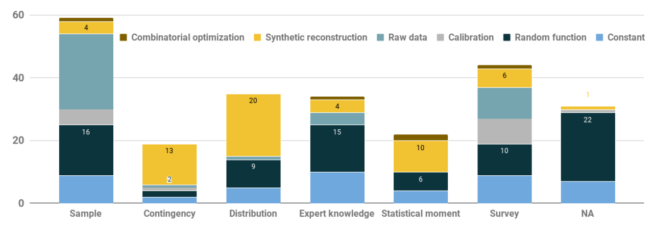
Another interesting outcome was the overall complexity of the generation procedure when modelers relied on rich data sources, such as samples and surveys. In these cases, the method to create the agents’ set of attributes was often a combination of two or three approaches among raw data, random function, constant values and SR techniques. When no data were used, modelers relied heavily on random functions (147, 42.98% of the corpus) and constant values (75, 21.92% of the corpus)
In addition to source data, we also correlated synthetic population generation processes with the use of GIS data and reports of a real-world case study application. In both cases, SR techniques were overrepresented, with 21.7% and 25% of models using these techniques to build the initial population of agents. If raw data and CO were included in the pool of established synthetic population techniques, half of the models associated with a real case study relied on these procedures. In terms of the use of data and GIS/real-world case studies, models more often built their synthetic population on refined techniques. Hence, the studied corpus tended to confirm Hypothesis H2: When modelers used data (including GIS data) and real-world applications, more models generated the synthetic population of agents with established procedures.
General trends over time and subdomains of the simulation models
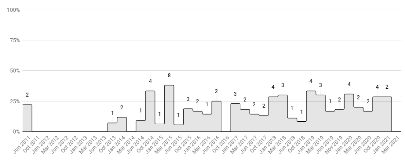
To examine the evolution of the use of synthetic populations, we correlated the descriptive statistics with years of publication and keywords. Figures 4 show the trend regarding both aspect of agent initialization: Figure 4a aggregates the proportion (number) of models that relied on real world data (all models except those with the NA and Expert knowledge code) per issue, while Figure 4b depicts the cumulative proportion (number) of models that used data to implement a known procedure in synthetic population generation (i.e., using either raw data, synthetic reconstruction or combinatorial optimization).
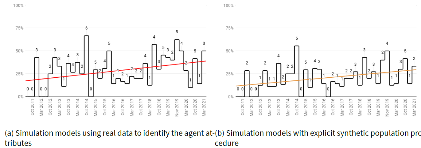
Despite the deviations, we observed a trend promoting the inclusion of data regarding targeted real population and explicit procedures related to synthetic population generation. Indeed, both the best fit linear regression models exhibited a gradual trend toward a more descriptive population of agents in models published in JASSS. However, comparison of the proportion of data used and actual use of well-established methodologies to construct the synthetic population of agents indicated a significant difference: on average 29.17% of the published models used conventional data regarding the target population, and only 22% relied on dedicated algorithm to generate synthetic population.
To link practices with sub-domains, we performed an occurrence-based analysis of terms in article keywords. Keywords can well approximate the subdomain as they are specified by the model developers. We identified each keyword as a token and collected occurrences for each model; all keywords similar to “agent-based model and simulation” were removed.
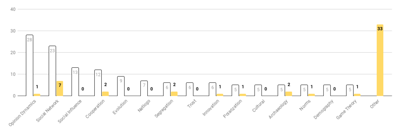
The results of the most mentioned keywords are plotted in Figure 5. Blank bars show the number of articles with corresponding keywords, while yellow bars display the subset of models using synthetic reconstruction. Opinion dynamics and social networks represented the most influential keyword in the journal, followed by more topic related items such as social influence, cooperation, segregation or trust. Except for social network-related models, most synthetic populations built using synthetic reconstruction did not pertain to the most prominent sub-domains of simulation studies in the journal.
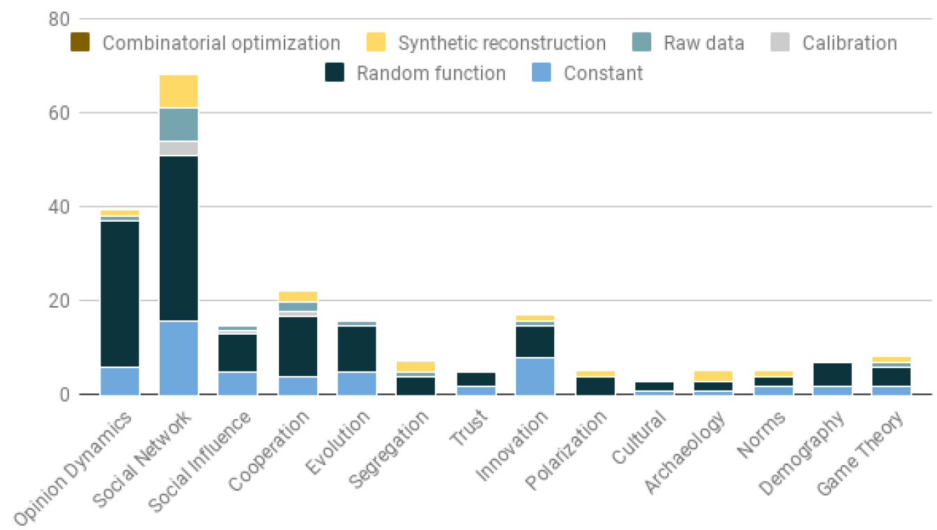
As shown in Figure 6 each synthetic population generation procedure was associated with the article keywords. The most influential themes in the corpus tended to use a random function or constant. Nonetheless, social network studies emphasized initialization, with an average of 2.56 distinct procedures used to generate the synthetic population of agent per model. These approaches often relied on a random function and constant. However, these approaches were driven by a clear tendency to comply with the available data (Section 4 on synthetic population and synthetic network).
Narrative review
As described here, we performed a more qualitative assessment of the reviewed articles. This narrative explanation of the field practices regarding synthetic population generation focused on three dimensions of the analyzed models: agent attributes and initialization, differences in these aspects for different types of models and actual methods to realize these aspects.
Description of the agent attributes and their initialization. The process used to generate the set of agents is often poorly described. This is alleviated by the use of the ODD protocol as it forces modelers to explicitly discuss the model initialization at the start of simulation and data used to implement the process. However, even though the adoption of standardized narratives to describe the early simulation step facilitates the identification of the key aspect of synthetic population generation, these narratives do not provide adequate guidance in this aspect. In this framework, the descriptions of different models are difficult to be compared. Identifying the method with which the modelers initialize the population of agents requires the examination of the source code when available. Similarly, a standard procedure regarding the description of the simulation experiment is lacking, even when the ODD protocol is used. For instance, in numerous examples (Chen et al. 2021; Houssou et al. 2019; Muelder & Filatova 2018; Xiong et al. 2018), it is difficult to identify the number of agents simulated and the number of time steps for which the simulation is performed, either because information is missing or because several values are specified for various experimental setups. Moreover, for clarity of the model presentation, the attribute descriptions do not match variable names in the model.
In all cases, basic information regarding the simulated agent properties cannot be extracted from articles as no standard methods are available to describe the model and simulation. The model, its implementation and the simulation experiments are three aspects of most reviewed models. Therefore, the description of these entities must be extensive to ensure that a reader can fill the gaps between these aspects. The synthetic population of agents lies between the model and simulation: The model defines the attributes that must be assigned to the agent, while simulation pertains to the initialization of values. In both cases, considerable work must be done to ensure that a reader can clearly observe how these aspects are managed, implemented and transformed to simulation results. Furthermore, for certain models, generation of the agent attributes is part of the simulation process or outcome of the model: Agents may be created during the simulation rather than in the initial stage (Houssou et al. 2019). In other cases, agent attributes must be generated by the model (Silverman et al. 2013).
Synthetic populations are not considered in all models. While descriptive ABMs with social entities fit our extraction framework, there is an important set of models ranging from extremely abstract agent-based models (e.g., bounded confidence and derivative models of opinion dynamics) to more classical agent-based systems (e.g., swarm or business process) in which the population generation is not of significance or ignored. The initial value of the agent attributes is often randomly drawn in an interval (using a uniform or Gaussian distribution) or simply not considered as important/relevant in the narrative of the model presentation. Even in the social simulation domain, having a coherent and well-generated synthetic population of agents is not mandatory in many cases. As mentioned previously, extremely abstract models subscribing to the KISS adage, and even models closer to the agent-based system paradigm do not seek to build a realistic set of agents in their experiment (one extreme example is presented in (Tang & Zeng 2018), in which an agent is not mentioned throughout the whole article).
However, the set of models that lies between abstract and descriptive models, among which the more popular models, such as opinion dynamics and game theoretical models, would benefit from using realistic synthetic populations of agents (Flache et al. 2017). For instance, considerable effort is expended in modeling realistic social networks while maintaining a low representativeness of the agent attributes. In general, abstract models tend to focus more on global or aggregated determinants of the considered implemented mechanisms (e.g., social influence, cooperation, segregation or trust) rather than determinants that lie within agents. In this regard, the status of agent attributes remains unclear, especially when compared to those of the inner state variables. Presumably, attributes to be generated in a synthetic population of agents pertain to a category of agent variables that drive the behavior and decisions of agents instead of being determined during the simulation. Hence, there exists a blurred distinction between agent attributes considered state variables (e.g., opinion in opinion dynamics models or utility in game theoretical models) and agent attributes as determinant variables. However, most of these determinant agent variables are inherently generated as a global property link to the relative position of agents, i.e., agents who the entities are connected either in a grid or a network.
Synthetic network generation. Most initial setups of agent attributes lie in their position in a network (or a simplified grid, which is simply used as a lattice considering a Moore or Von Neumann neighborhood), with most effort being focused on synthetic network generation. The position of the agent may be considered partly as an attribute (e.g., agent’s living address) and partly as an environmental feature (e.g., the distance between agents is defined by an underlying grid). In most cases, the second option is chosen, and parameters and/or data used to generate the synthetic network express aggregated characteristics rather than local properties or agent attributes. There is a set of models that should be attached to the network model rather than ABM, with most “agent” (node) attributes being related to their ties.
Discussion
A key issue related to the generation of a set of agents is defining the scope and problem of the synthetic population. In most cases, the problem is not well defined; e.g., not all models require a heavily data-oriented synthetic population generation process, whereas models disregarding this aspect can consider the use of simple yet dedicated sub-models for synthetic population generation. Global disinterest in the established approach can be attributed to this low expectancy regarding the realism of agents. However, we recommend the examination of the limited use in terms of the accessibility: (i) methods may not be well understood because the domain of synthetic population may involve ambiguities (Section 2.2) and dispersion of the proposed methodologies; (ii) available tools are difficult to find and adapt to a particular case study; and (iii) tools may not be incorporated in the platform used to implement models and conduct simulation experiments, which renders the inclusion of the tools in the simulation pipeline challenging.
In addition to the neglect of the synthetic population generation procedure, there are issues related to the description of agent creation and agent attribute definitions. While the use of ODD can enhance the reusability and replicability of models, the initialization step remains a bottleneck to the model description.
- Conflict within ODD between initialization (what is the process to build all the elements needed for the model simulation) and data (how are the processes of the model, rather than agent attributes, based on data? What is the influence of the initial value for a changing attributes?)
- Models often rely on a constellation of loosely categorized inputs generalized into a parameter or data dichotomy, while there exist constants, parameters for the simulation, environment (global) and agents (local), attributes and inner states of agents, and raw and preprocessed data, among other types of inputs.
Thus, the ODD is generally not enough to be able to understand how agent populations are initialized in the models. Following recommendations by Müller et al. (2014), a minimum standard must be established, which consists of a structured natural language description such as ODD and source code.
The source code is often easy to interpret and understand depending on the language / platform / toolkit used. Notably, it is considerably easier to understand a noncompiled and readable code (text file) developed with an agent-oriented language (Netlogo, GAMA, etc.) or an object-oriented language
Within the scope of this review, the limited search for a specific journal involves certain biases. In particular, several well-known references cited in the first part of the paper come from a related field of research, i.e., transport modeling. Such models might be under-represented in JASSS while at the same time, considerably influencing how researchers generate synthetic populations for use in ABM. It would be interesting to focus on simulation models published in journals such as Transportation Research, for instance, to gain knowledge regarding practices from a related field. As kindly stated by a reviewer of this paper, "the strategy of basing a review around material in JASSS made reasonable sense in view of the importance of the journal and its large canon of relevant literature". We believe JASSS offers a relatively free of domain view on practices related to ABM, although future work should be focused on synthetic population generation for other types of simulation models, such as microsimulations. In summary, outcomes from practices in JASSS cannot be generalized to ABM, especially when simulation models use mixed modeling techniques, which is often the case in transport modeling research but also and more recently in epidemiological research.
We did not perform a systematic review due to the initial results that we obtained from a systematic search: in the ABM domain, synthetic population represents a sub-field. In other words, for the search based on general purpose searching tools such as Google Scholar, semantic Scholar or Scopus, and dedicated search engines, such as iris.ai, most of the results were concerned with methodological aspects, i.e., proposal of a procedure to generate a synthetic population instead of that of a model featuring a synthetic population generation. The outcome of a systematic search, although interesting when studying synthetic population procedures, did not reflect our subject of interest: actual synthetic population generation processes in agent-based simulation models. To review the practices, we were required to review the simulation models more broadly. To ensure manageability, we therefore selected a specific journal.
Conclusion
Despite the trend toward integration of realistic synthetic populations of agents, our review underlines several practical biases in the domain. We observe that models are tending to integrate increasingly more data but disregarding the proposed methodologies to guide the creation of agents. Our investigation validates Hypothesis H-1: the use of the synthetic population generation approach is still uncommon in social simulation. Specifically, modelers more often use generic purpose initialization procedures such as the assignment of constant values or sampling from a given continuous distribution (H-1b). While data regarding the target population remain of limited use (H-1a), an increasing number of models are driving the generation of agents attributed to them. Finally, we identify disparities in practices according to the modeling target: when models are attached to real-world applications, they more frequently apply well-established synthetic population generation methodologies (H-2).
Several hypotheses can be made to explain this state. The first aspect is the lack of data concerning several attributes, in particular, the abstract attributes related to social attitudes and mental states render it impossible to consider all agent attributes using the current synthetic population generation procedure. Another aspect is the lack of knowledge and control of the population generation approaches by modelers: in this case, modelers rely heavily on simple random methods such as uniform sampling of attribute values. Even if we consider that dedicated methodologies are available and known by most modelers, there remains a lack of accessibility because a specific tool (usually, an API) or programming language (such as R, Python or Java) must be used, which differs from the one used to implement the model and conduct experiments.
Considering these aspects, we have outlined several ways to foster the use of dedicated methods to build a realistic set of agents and describe how the synthetic population is built in simulation models. First, the proposed methodologies presented in the first section must truly focus on data harmonization and integration of agent population synthesis). Furthermore, the models must use easy-to-couple software with simulation tools in the form of plugins for generic platforms or comprehensive APIs. From the modeler viewpoint, enhancement of the model description, in particular, the data and initialization step of simulation experiments, can enable the identification of appropriate features and tools to address various requirements in terms of synthetic population. Not all models require the same type of agent population, although little is known regarding the diversity of goals and the extent to which the agent must be realistic. While considerable effort has been expended to generate realistic social networks, future work must focus on establishing reliable and reproducible synthetic populations in social simulations.
Acknowledgements
This work is part of the GEN* research project funded by the French National Research Agency. We wish to thank EIFER, and, especially, Samuel Thiriot, for his participation in the funding of the research associated with the generation of synthetic populations.Notes
- 2 of the 30 first results also pertain to a different use of synthetic population in biology.↩︎
- NA denotes unattributed and represents either a lack of information or the absence of algorithms/data used.↩︎
- Access to the file and explicit url can be requested if the link if broken.↩︎
Appendix
Appendix A: Codebook Guidelines
Guidelines for the content extraction process were established with reference to a preliminary study (Chapuis & Taillandier 2019) and exploratory content extraction over the 4 last issues.
Content extraction guidelines
- Q1 - Does the article present a synthetic population generation model? [yes/no]
- Q2 - Is a simulation model described in the article? [yes/no]
- Q3 - Is there an ODD that describes the simulation model? [yes/no]
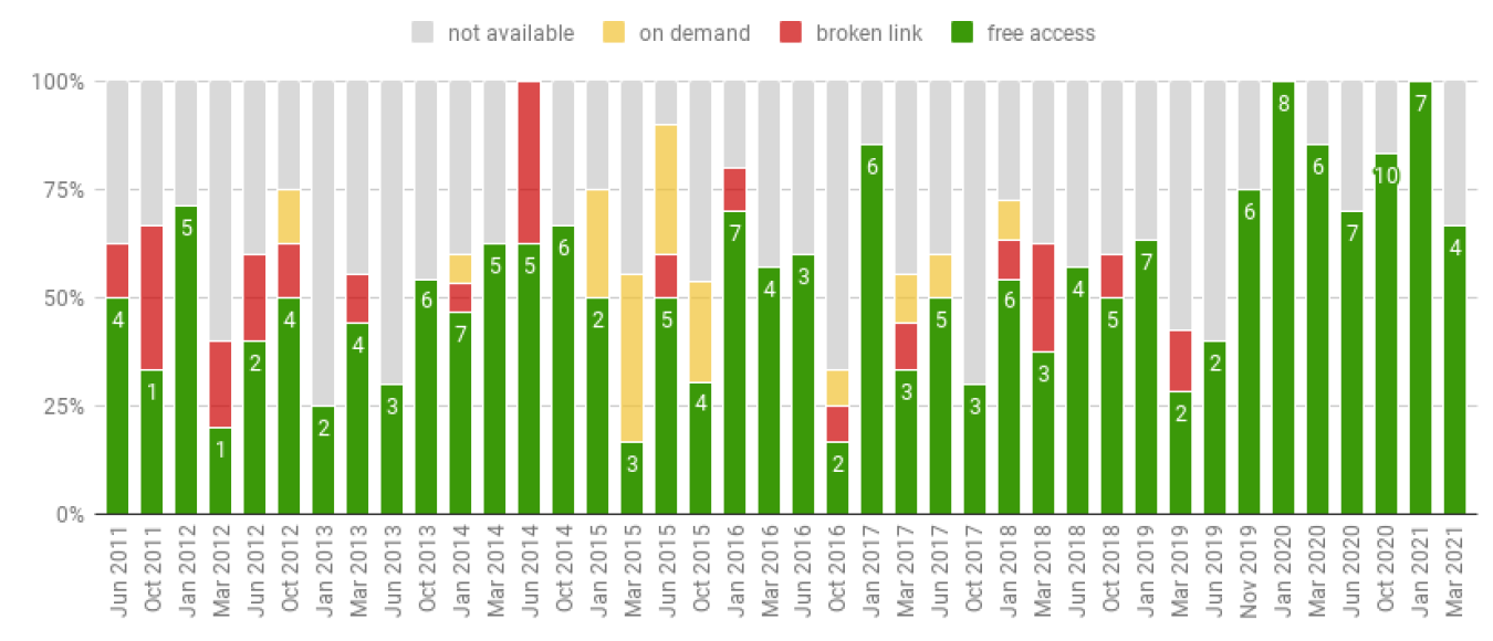
- Q4 - Is the code accessible? [free access/on demand/not available]
- Q5 - Use case
- Q5.1 - What is the location represented in the simulation model? [Free text]
- Q5.2 - What time is the simulated case study associated with? [Free text]
- Q5.3 - Do modelers use GIS data in the simulation model? [yes/no]
- Q6 - Entities and attributes
- Q6.1 - What are the principal entities (i.e., more than one and active agents) generated at the initialization of the simulation? [Free text]
- Q6.2 - How many entities are generated? [Number per type of entities]
- Q6.3 - List of attributes (with types) for each generated entity [List]
- Q7 - What are the algorithms/techniques used to generate the attribute values? see subsection below
- Q8 - Input Data
- Q8.1 - Are empirical data used? [yes/no]
- Q8.2 - What kind of data is used? see subsection below
- Q8.3 - Source of data [Free text]
Categories of synthetic population generation procedure (Q7)
- Constant: fixed attribute value
- Raw data: attribute value directly extracted from the data sources
- Random function: attribute value specified by a generic continuous function
- Calibration: attribute value based on the optimization of the simulated results
- Synthetic reconstruction: attribute value based on a random engine calibrated on population data (Section 2)
- Combinatorial optimization: attribute value drawn with replacement from a known real individual (Section 2)
- NA: unclear or unknown procedure to assign attribute values
Categories of input data type to implement synthetic population generation (Q8.2)
- Sample: equivalent to microdata (Subsection 2.8)
- Contingency: aggregated data regarding the population in the form of counts of corresponding people, e.g., the number of men and women (Subsection 2.8)
- Distribution: aggregated data regarding the population in the form of proportion, e.g,. percentage of people aged under 16 (Subsection 2.8)
- Statistical moment: aggregated data about population in the form of a synthetic statistical indicator, e.g. mean age of the population (Subsection 2.8)
- Expert knowledge: second-hand information without a clearly identified source of data
- Survey: social endeavor in the form of a questionnaire, direct observation or any participatory survey focused on a particular subject, e.g., time use survey, in which people are asked to describe in a closed form how their schedule is actually organized, see, for instance, Eurostats: https://ec.europa.eu/eurostat/web/microdata/time-use-survey.
Appendix B: Codebook
The raw data results are stored in a Google sheets with public access here: https://docs.google.com/spreadsheets/d/1Aj_WU7jlcyYQKbe8_sJFYL0GlDxsGZljzXBfCw9zMxY/edit?usp=sharing.3 The first sheet describes the screening and eligibility of articles as well as extraction content based on codebook guidelines. All other sheets are dedicated to the analysis, facilitating the verification and reproduction of published results. A pdf (csv) version of the codebook itself can be accessed here: https://drive.google.com/file/d/1L2BgJ0ThhIirI0TJVDQhlRgJuGLrNwNw/view?usp=sharing (here: https://drive.google.com/file/d/1ryug3b3nW_3TwdRIay6PomV_WPKAh8UV/view?usp=sharing).
References
AMBLARD, F., Bouadjio-Boulic, A., Sureda Gutierrez, C., & Gaudou, B. (2015). Which models are used in social simulation to generate social networks? A review of 17 years of publications in JASSS. Proceedings of the 2015 Winter Simulation Coference, Huntington Beach, California. Available at: https://hal.archives-ouvertes.fr/hal-01303799/document. [doi:10.1109/wsc.2015.7408556]
AXELROD, R. M. (1997). The Complexity of Cooperation: Agent-Based Models of Competition and Collaboration. Princeton, NJ: Princeton University Press. [doi:10.1515/9781400822300]
BARTHELEMY, J., & Toint, P. L. (2012). Synthetic population generation without a sample. Transportation Science, 47(2), 266–279. [doi:10.1287/trsc.1120.0408]
BECKMAN, R. J., Baggerly, K. A., & McKay, M. D. (1996). Creating synthetic baseline populations. Transportation Research Part A: Policy and Practice, 30(6), 415–429. [doi:10.1016/0965-8564(96)00004-3]
BOURGAIS, M., Taillandier, P., & Vercouter, L. (2020). BEN: An architecture for the behavior of social agents. Journal of Artificial Societies and Social Simulation, 23(4), 12: https://www.jasss.org/23/4/12.html. [doi:10.18564/jasss.4437]
CASATI, D., Müller, K., Fourie, P. J., Erath, A., & Axhausen, K. W. (2015). Synthetic population generation by combining a hierarchical, simulation-Based approach with reweighting by generalized raking. Transportation Research Record: Journal of the Transportation Research Board, 2493, 107–116. [doi:10.3141/2493-12]
CHAPUIS, K., & Taillandier, P. (2019). A brief review of synthetic population generation practices in agent-based social simulation. Social Simulation Conference 2019, Mainz, Germany.
CHATTOE-BROWN, E. (2014). Using agent based modelling to integrate data on attitude change. Sociological Research Online, 19(1), 159–174. [doi:10.5153/sro.3315]
CHEN, Y., Irwin, E., Jayaprakash, C., & Park, K. J. (2021). An agent based model of a thinly traded land market in an urbanizing region. Journal of Artificial Societies and Social Simulation, 24(2), 1: https://www.jasss.org/24/2/1.html. [doi:10.18564/jasss.4518]
CHOUPANI, A. A., & Mamdoohi, A. R. (2016). Population synthesis using iterative proportional fitting (IPF): A review and future research. Transportation Research Procedia, 17, 223–233. [doi:10.1016/j.trpro.2016.11.078]
DUMONT, M., Barthelemy, J., Huynh, N. N., & Carletti, T. (2018). Towards the right ordering of the sequence of models for the evolution of a population using agent-based simulation. Journal of Artificial Societies and Social Simulation, 21(4), 3: https://www.jasss.org/21/4/3.html. [doi:10.18564/jasss.3790]
EDMONDS, B., & Moss, S. (2005). 'From KISS to KIDS - An “Anti-simplistic” modelling approach.' In P. Davidsson, B. Logan, & K. Takadama (Eds.), Multi-Agent and Multi-Agent-Based Simulation (pp. 130–144). Berlin Heidelberg: Springer. [doi:10.1007/978-3-540-32243-6_11]
FAROOQ, B., Bierlaire, M., Hurtubia, R., & Flötteröd, G. (2013). Simulation based population synthesis. Transportation Research Part B: Methodological, 58, 243–263. [doi:10.1016/j.trb.2013.09.012]
FELBERMAIR, S., Lammer, F., Trausinger-Binder, E., & Hebenstreit, C. (2020). Generation of a synthetic population for agent-based transport modelling with small sample travel survey data using statistical raster census data. International Journal of Traffic and Transportation Management, 02(02), 9–17. [doi:10.5383/jttm.02.02.002]
FLACHE, A., Mäs, M., Feliciani, T., Chattoe-Brown, E., Deffuant, G., Huet, S., & Lorenz, J. (2017). Models of social influence: Towards the next frontiers. Journal of Artificial Societies and Social Simulation, 20(4), 2: https://www.jasss.org/20/4/2.html. [doi:10.18564/jasss.3521]
GALLAGHER, S., Richardson, L., Ventura, S. L., & Eddy, W. F. (2018). SPEW: Synthetic Populations and Ecosystems of the World. Journal of Computational and Graphical Statistics, 27(4), 773–784. [doi:10.1080/10618600.2018.1442342]
GARGIULO, F., Ternes, S., Huet, S., & Deffuant, G. (2010). An iterative approach for generating statistically realistic populations of households. PLoS ONE, 5(1), e8828. [doi:10.1371/journal.pone.0008828]
GARRIDO, S., Borysov, S. S., Pereira, F. C., & Rich, J. (2020). Prediction of rare feature combinations in population synthesis: Application of deep generative modelling. Transportation Research Part C: Emerging Technologies, 120, 102787. [doi:10.1016/j.trc.2020.102787]
GORE, R., Lemos, C., Shults, F. L., & Wildman, W. J. (2018). Forecasting changes in religiosity and existential security with an agent-Based model. Journal of Artificial Societies and Social Simulation, 21(1), 4. [doi:10.18564/jasss.3596]
GRIMM, V., Berger, U., DeAngelis, D. L., Polhill, J. G., Giske, J., & Railsback, S. F. (2010). The ODD protocol: A review and first update. Ecological Modelling, 221(23), 2760–2768. [doi:10.1016/j.ecolmodel.2010.08.019]
GUO, J., & Bhat, C. (2007). Population synthesis for microsimulating travel behavior. Transportation Research Record: Journal of the Transportation Research Board, 2014(1), 92–101. [doi:10.3141/2014-12]
HAFEZI, M. H., & Habib, M. A. (2014). Synthesizing population for microsimulation-based integrated transport models using Atlantic Canada micro-data. Procedia Computer Science, 37, 410–415. [doi:10.1016/j.procs.2014.08.061]
HARLAND, K., Heppenstall, A., Smith, D., & Birkin, M. (2012). Creating realistic synthetic populations at varying spatial scales: A comparative critique of population synthesis techniques. Journal of Artifical Societies and Social Simulation, 15(1), 1: https://www.jasss.org/15/1/1.html. [doi:10.18564/jasss.1909]
HOERTEL, N., Blachier, M., Blanco, C., Olfson, M., Massetti, M., Rico, M. S., Limosin, F., & Leleu, H. (2020). A stochastic agent-based model of the SARS-CoV-2 epidemic in France. Nature Medicine, 26, 1417–1421. [doi:10.1038/s41591-020-1001-6]
HOUSSOU, N. L. J., Cordero, J. D., Bouadjio-Boulic, A., Morin, L., Maestripieri, N., Ferrant, S., Belem, M., Pelaez Sanchez, J. I., Saenz, M., Lerigoleur, E., Elger, A., Gaudou, B., Maurice, L., & Saqalli, M. (2019). Synchronizing histories of exposure and demography: The construction of an agent-Based model of the Ecuadorian Amazon Colonization and exposure to oil pollution hazards. Journal of Artificial Societies and Social Simulation, 22(2), 1: https://www.jasss.org/22/2/1.html. [doi:10.18564/jasss.3957]
HUANG, Z., & Williamson, P. (2001). A comparison of synthetic reconstruction and combinatorial optimisation approaches to the creation of small-area microdata. Working Paper, Department of Geography, University of Liverpool. Available at: http://pcwww.liv.ac.uk/~william/microdata/workingpapers/hw_wp_2001_2.pdf. [doi:10.1007/978-94-007-4623-7_3]
HUYNH, N., Barthelemy, J., & Perez, P. (2016). A heuristic combinatorial optimisation approach to synthesising a population for agent based modelling purposes. Journal of Artificial Societies and Social Simulation, 19(4), 11: https://www.jasss.org/19/4/11.html. [doi:10.18564/jasss.3198]
JAGER, W. (2017). Enhancing the realism of simulation (EROS): On implementing and developing psychological theory in social simulation. Journal of Artificial Societies and Social Simulation, 20(3), 14. [doi:10.18564/jasss.3522]
JEONG, B., Lee, W., Kim, D.-S., & Shin, H. (2016). Copula-Based approach to synthetic population generation. PLoS ONE, 11(8), e0159496. [doi:10.1371/journal.pone.0159496]
KIM, J., & Lee, S. (2015). A reproducibility analysis of synthetic population generation. Transportation Research Procedia, 6, 50–63. [doi:10.1016/j.trpro.2015.03.005]
KURBAN, H., Gallagher, R., KURBAN, G. A., & Persky, J. (2011). A beginner’s guide to creating small-area cross-tabulations. Cityscape, 13(3), 225–235.
LENORMAND, M., & Deffuant, G. (2013). Generating a synthetic population of individuals in households: Sample-Free Vs sample-Based methods. Journal of Artificial Societies and Social Simulation, 16(4), 12: https://www.jasss.org/16/4/12.html. [doi:10.18564/jasss.2319]
LOVELACE, R., Birkin, M., Ballas, D., & van Leeuwen, E. (2015). Evaluating the performance of iterative proportional fitting for spatial microsimulation: New tests for an established technique. Journal of Artificial Societies and Social Simulation, 18(2), 21: https://www.jasss.org/18/2/21.html. [doi:10.18564/jasss.2768]
MA, L., & Srinivasan, S. (2015). Synthetic population generation with multilevel controls: A fitness-Based synthesis approach and validations. Computer-Aided Civil and Infrastructure Engineering, 30(2), 135–150. [doi:10.1111/mice.12085]
MOECKEL, R., Spiekermann, K., & Wegener, M. (2003). Creating a synthetic population. Proceedings of the 8th International Conference on Computers in Urban Planning and Urban Management (CUPUM).
MOHER, D., Liberati, A., Tetzlaff, J., & Altman, D. G. (2009). Preferred reporting items for systematic reviews and meta-Analyses: The PRISMA statement. PLoS Medicine, 6(7), e1000097. [doi:10.1371/journal.pmed.1000097]
MUELDER, H., & Filatova, T. (2018). One theory - many formalizations: Testing different code implementations of the theory of planned behaviour in energy agent-Based models. Journal of Artificial Societies and Social Simulation, 21(4), 5: https://www.jasss.org/21/1/5.html. [doi:10.18564/jasss.3855]
MÜLLER, B., Balbi, S., Buchmann, C. M., De Sousa, L., Dressler, G., Groeneveld, J., Klassert, C. J., Le, Q. B., Millington, J. D., Nolzen, H., Parker, D. C., Polhill, J. G., Schlüter, M., Schulze, J., Schwarz, N., Sun, Z., Taillandier, P., & Weise, H. (2014). Standardised and transparent model descriptions for agent-based models: Current status and prospects. Environmental Modelling & Software, 55, 156–163.
MÜLLER, K., & Axhausen, K. W. (2010). Population synthesis for microsimulation: State of the art. ETH Zürich, Institut für Verkehrsplanung, Transporttechnik, Strassen-und Eisenbahnbau (IVT).
MÜLLER, K., & Axhausen, K. W. (2011). Hierarchical IPF: Generating a synthetic population for Switzerland. Available at: http://www-sre.wu.ac.at/ersa/ersaconfs/ersa11/e110830aFinal00305.pdf.
OTANI, N., Sugiki, N., & Miyamoto, K. (2010). Goodness-of-fit evaluation method between two sets of household micro-data for land-use microsimulation model. Selected Proceedings of 12th WCTR.
RYAN, J., Maoh, H., & Kanaroglou, P. (2009). Population synthesis: Comparing the major techniques using a small, complete population of firms. Geographical Analysis, 41(2), 181–203. [doi:10.1111/j.1538-4632.2009.00750.x]
SAID, L. B., Bouron, T., & Drogoul, A. (2002). Agent-based interaction analysis of consumer behavior. Proceedings of the First International Joint Conference on Autonomous Agents and Multiagent Systems: Part 1. Available at: https://www.researchgate.net/profile/Alexis-Drogoul/publication/221455937. [doi:10.1145/544741.544787]
SILVERMAN, E., Bijak, J., Hilton, J., Cao, V. D., & Noble, J. (2013). When demography met social simulation: A tale of two modelling approaches. Journal of Artificial Societies and Social Simulation, 16(4), 9: https://www.jasss.org/16/4/9.html. [doi:10.18564/jasss.2327]
SMITH, A., Lovelace, R., & Birkin, M. (2017). Population synthesis with quasirandom integer sampling. Journal of Artificial Societies and Social Simulation, 20(4), 14: https://www.jasss.org/20/4/14.html. [doi:10.18564/jasss.3550]
SRINIVASAN, S., Ma, L., & Yathindra, K. (2008). Procedure for forecasting household characteristics for input to travel-demand models. Working Paper Florida Department of Transportation, University of Florida, Gainesville. Available at: http://www.fsutmsonline.net/images/uploads/reports/FDOTBD54579rpt.pdf.
STEPHAN, F. F. (1942). An iterative method of adjusting sample frequency tables when expected marginal totals are known. The Annals of Mathematical Statistics, 13(2), 166–178. [doi:10.1214/aoms/1177731604]
SUN, L., & Erath, A. (2015). A Bayesian network approach for population synthesis. Transportation Research Part C: Emerging Technologies, 61, 49–62. [doi:10.1016/j.trc.2015.10.010]
SUN, L., Erath, A., & Cai, M. (2018). A hierarchical mixture modeling framework for population synthesis. Transportation Research Part B: Methodological, 114, 199–212. [doi:10.1016/j.trb.2018.06.002]
TAGHIKHAH, F., Filatova, T., & Voinov, A. (2021). Where does theory have it right? A comparison of theory-Driven and empirical agent based models. Journal of Artificial Societies and Social Simulation, 24(2), 4: https://www.jasss.org/24/2/4.html. [doi:10.18564/jasss.4573]
TANG, T., & Zeng, K. (2018). Evolution of government’s performance through yardstick competition in the spatial game of gubernatorial elections. Journal of Artificial Societies and Social Simulation, 21(2), 7: https://www.jasss.org/21/2/7.html. [doi:10.18564/jasss.3624]
TANTON, R., Williamson, P., & Harding, A. (2014). Comparing two methods of reweighting a survey file to small area data. International Journal of Microsimulation, 7(1), 76–99. [doi:10.34196/ijm.00094]
THIELE, J. C., Kurth, W., & Grimm, V. (2014). Facilitating parameter estimation and sensitivity analysis of agent-Based models: A cookbook using NetLogo and ’R’. Journal of Artificial Societies and Social Simulation, 17(3), 11: https://www.jasss.org/17/3/11.html. [doi:10.18564/jasss.2503]
THIRIOT, S., & Kant, J.-D. (2008). Generate country-scale networks of interaction from scattered statistics. The Fifth Conference of the European Social Simulation Association, Brescia, Italy.
THIRIOT, S., & Sevenet, M. (2020). Pairing for generation of synthetic populations: The direct probabilistic pairing method. arXiv preprint. Available at: https://arxiv.org/abs/2002.03853.
TIMMINS, K. A., & Edwards, K. L. (2016). Validation of spatial microsimulation models: A proposal to adopt the Bland-Altman method. Available at: https://microsimulation.pub/articles/00137. [doi:10.34196/ijm.00137]
VOAS, D., & Williamson, P. (2000). An evaluation of the combinatorial optimisation approach to the creation of synthetic microdata. International Journal of Population Geography, 6(5), 349–366. [doi:10.1002/1099-1220(200009/10)6:5<349::aid-ijpg196>3.0.co;2-5]
WATTHANASUTTHI, N., & Muangsin, V. (2016). Generating synthetic population at individual and household levels with aggregate data. IEEE. Available at: https://ieeexplore.ieee.org/document/7748838. [doi:10.1109/jcsse.2016.7748838]
WICKRAMASINGHE, B. N. (2019). Application independent heuristic data merging methodology for sample-Free agent population synthesis. Journal of Artificial Societies and Social Simulation, 22(1), 5: https://www.jasss.org/22/1/5.html. [doi:10.18564/jasss.3844]
WILLIAMSON, P. (2012). 'An evaluation of two synthetic small-area microdata simulation methodologies: Synthetic reconstruction and combinatorial optimisation.' In R. Tanton & K. Edwards (Eds.), Spatial Microsimulation: A Reference Guide for Users (pp. 19–47). Berlin Heidelberg: Springer. [doi:10.1007/978-94-007-4623-7_3]
WILLIAMSON, P., Birkin, M., & Rees, P. H. (1998). The estimation of population microdata by using data from small area statistics and samples of anonymised records. Environment and Planning A, 30(5), 785–816. [doi:10.1068/a300785]
WILSON, A. G., & Pownall, C. E. (1976). A new representation of the urban system for modelling and for the study of micro-level interdependence. Area, 8(4), 246–254.
XIONG, H., Payne, D., & Kinsella, S. (2018). Identifying mechanisms underlying peer effects on multiplex networks. Journal of Artificial Societies and Social Simulation, 21(4), 6: https://www.jasss.org/21/4/6.html. [doi:10.18564/jasss.3797]
YAMEOGO, B. F., Vandanjon, P.-O., Gastineau, P., & Hankach, P. (2021). Generating a two-Layered synthetic population for French municipalities: Results and evaluation of four synthetic reconstruction methods. Journal of Artificial Societies and Social Simulation, 24(2), 5: https://www.jasss.org/24/2/5.html. [doi:10.18564/jasss.4482]
YE, P., Hu, X., Yuan, Y., & Wang, F.-Y. (2017). Population synthesis based on joint distribution inference without disaggregate samples. Journal of Artificial Societies and Social Simulation, 20(4), 16: https://www.jasss.org/20/4/16.html. [doi:10.18564/jasss.3533]
YE, P. J., Wang, X., Chen, C., Lin, Y. T., & Wang, F. Y. (2016). Hybrid agent modeling in population simulation: Current approaches and future directions. Journal of Artificial Societies and Social Simulation, 19(1), 12: https://www.jasss.org/19/1/12.html. [doi:10.18564/jasss.2849]
YE, X., Konduri, K., Pendyala, R. M., Sana, B., & Waddell, P. (2009). A methodology to match distributions of both household and person attributes in the generation of synthetic populations. 88th Annual Meeting of the Transportation Research Board, Washington, DC.
ZHU, Y., & Ferreira, J. (2014). Synthetic population generation at disaggregated spatial scales for land use and transportation microsimulation. Transportation Research Record: Journal of the Transportation Research Board, 2429, 168–177. [doi:10.3141/2429-18]
ZIEMKE, D., Nagel, K., & Moeckel, R. (2016). Towards an agent-based, integrated land-use transport modeling system. Procedia Computer Science, 83(2016), 958–963. [doi:10.1016/j.procs.2016.04.192]