Effect of Policy Implementation on Energy Retrofit Behavior and Energy Consumption in a Simulated Neighborhood

and
aNorwegian University of Science and Technology, Norway; bNTNU - Norges Teknisk-Naturvitenskaplige Universitet, Norway
Journal of Artificial
Societies and Social Simulation 25 (4) 7
<https://www.jasss.org/25/4/7.html>
DOI: 10.18564/jasss.4936
Received: 12-Aug-2021 Accepted: 18-Oct-2022 Published: 31-Oct-2022
Abstract
As the heating of private households represents 16.5% of all EU final energy consumption, household energy retrofitting is a central part of the solution for the ongoing climate crisis. However, ABM models have not sufficiently been explored as a tool for designing policies for reducing household heating energy consumption through energy retrofitting. This paper presents the Household Energy Retrofit Behavior (HERB) model, which simulated energy retrofitting in a neighbourhood. The HERB model feeds a decision-making process based on existing behavioural household retrofit research with survey data and assesses the impact of different policies on cumulative energy need over 100 years. The model finds that the current Norwegian main retrofit subsidies have a positive effect on energy use. Furthermore, although motivating households to retrofit to a specific standard has no positive impact, motivating households close to retrofitting has a positive effect. Finally, lowering the threshold for receiving subsidies has a positive impact.Introduction
Sustainable development meets the needs of the present without compromising the ability of future generations to meet their own needs (United Nations - UN 1987). Central to achieving this goal is reducing global energy consumption. In the EU, 16.5% of final energy consumption is used for private household space heating (Eurostat 2019). Energy retrofitting is seen as the best way to reduce household energy consumption (Verbeeck & Hens 2005), and both large-scale research projects (e.g., the European Renovation Wave; European Commission 2020) and numerous governmental policies (Federal Office for the Environment 2018; Fyhn et al. 2019) are in place to find ways to increase the rate to which households retrofit. The importance of energy retrofit policies has resulted in a large share of research from both the fields of economics (Galvin & Sunikka-Blank 2013; Hill 2019), psychology (Klöckner & Nayum 2016), and others (Gillard et al. 2017).
Apart from this empirical and theoretical work, the issue of energy retrofits has also been addressed from a social simulation perspective. In this line of research, a number of agent-based models (ABM) have been proposed to assist policymaking on private household energy retrofitting. One of them, the ‘Neighbor Influenced Energy Retrofit’ (NIER) ABM, simulates a neighbourhood where opinion leaders, conformists, and stigma-avoiding households make retrofit decisions. Results from the NIER model suggest that forming building owner associations and energy efficiency organizations to leverage peer influence should positively affect household energy standards (Boria 2020b, 2020a). In a second model, Friege et al. (2016) populated a simulated neighbourhood with homeowners in categories based on Otte’s lifestyle typology for Germany (Otte 2008), where agents start thinking about renovating if certain conditions are triggered. Their model suggests that instead of going directly to homeowners, policymakers should incentivize lenders and artisans to advise homeowners to add insulation. A third ABM simulating buildings, governments, house owners, and environmental factors investigated different subsidy models for Chinese energy retrofit subsidy rates (Liang et al. 2019). They found that targeting subsidy levels in relation to energy prices and owner characteristics could significantly improve the current subsidy policy.
Although we think these models make a solid contribution to the field, we argue that the range of existing models has not yet fully explored the different ways of modelling the phenomenon. For example, both Friege et al. (2016) and the NIER divide households into categories such as leader or conformists. But as far as we are aware, most energy retrofitting behavioural research bases itself on independent continuous scales and not nominal categories such as leaders or conformists (Egner et al. 2021; Egner & Klöckner 2021; Klöckner & Nayum 2016; Nair et al. 2010). Although some categorical aspects are used (e.g. Klöckner & Nayum 2016), we argue that, in general, heavy utilization of categorical systems is a sign of not sufficiently basing models in existing litterature. While a model where all agents have several independent continuous variables will be more chaotic and ‘black-boxy’ where the causal inference is harder to pin down, this tradeoff is yet to be explored. Importing survey data and allowing each agent to represent one random participant should be a way of exploring such a setup.
Additionally, relying on more commonly established energy efficiency metrics such as \(kWh\)/(\(m^{2}a\)) instead of 0-100% scores of how energy efficient the building is, has not been explored. This omission is likely because ABMs focused on the behaviour of energy retrofitting do not have the resources to create an accurate technical representation of the energy standard of households. Therefore, it could be seen as better to implement an arbitrary scale, than a detailed but incorrect scale. Still, this makes tasks such as implementing other research findings (e.g. cost of energy retrofitting; Galvin 2010), integrating with other research (e.g., energy system models) and interpreting the effectiveness of policies difficult. While an arbitrary value is a more accurate representation of such a value, an exact value makes the transition to other research more seamless.
To further explore how ABMs can contribute to the energy retrofitting literature, we aimed to create a new model based on existing psychologically informed research regarding private household’s energy retrofitting behaviour (see below for the used research papers), which uses established energy metrics as one type of outputs to be compatible with models of the energy system and the policy debate, and base the agents on individual responses to representative surveys. This model has two goals. First, we aim to replicate retrofit rates, free-rider rates, and consecutive retrofitting rates reported for the same region in other research (Egner et al. 2021; Egner & Klöckner 2021; Fyhn et al. 2019) to validate the underlying model assumptions. These will be explained in Section 2.3. Second, we aim to assess current and planned Norwegian energy retrofitting policies on total household energy consumption and use the model as a testbed for alternative policy scenarios. In this paper, we present the model architecture, the model validation step, and some first takes on step two of the research (policy scenarios) to demonstrate the model’s abilities.
The Agent-Based Model
To address these objectives, we created the Household Energy Retrofit Behavior (HERB) model, where households conduct energy retrofits based on a 4 stage decision-making model in a simulated neighbourhood. The complete model, alongside an Overview, Design concepts, Details report (Grimm et al. 2006; Polhill et al. 2008), data output files from all experiments, and the syntax for the statistical analysis of these experiments can be downloaded from CoMSES: https://www.comses.net/codebases/72d1d19f-1fd5-463f-8cf3-ba13f26d4fa6.
Input data
The model uses input data from two surveys distributed to representative samples of Norwegian households between January and March 2014 and between March and April 2019. The surveys had 2,605 and 3,797 respondents, respectively, and were pooled, forming a total sample of 6,402 respondents. The first sample is the same as the parameterization sample used in Klöckner & Nayum (2016). Most data initializing the households were a direct representation of participants in these surveys. As the surveys originally had missing data, multiple imputations were used to impute missing data. See the ODD protocol for details regarding this imputation.
Overview
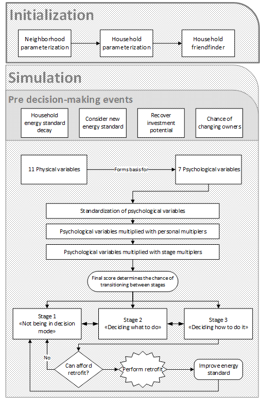
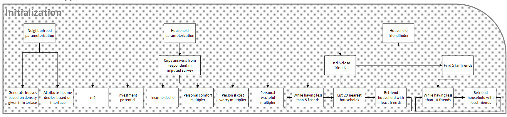
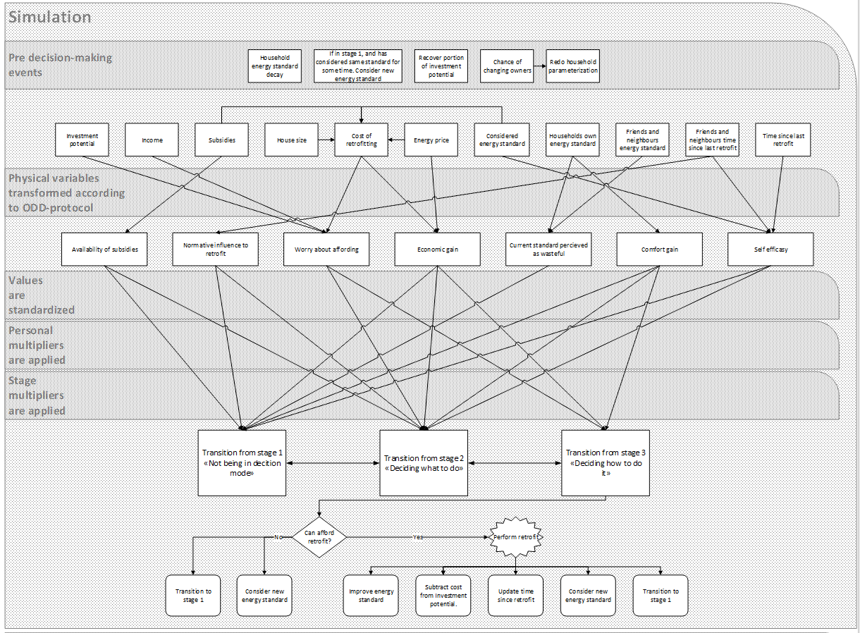
The HERB model simulates the retrofit behaviour of homeowners in a neighbourhood. The model initially parameterizes a neighbourhood and households with technical factors such as energy standard, the availability of subsidies, and neighbours’ retrofit activity. Then, these factors are translated into psychological variables such as perceived thermal comfort gain due to an improved energy standard, worry about affording the retrofit, and perceiving the current energy standard of the home as wasteful. These psychological variables moderate the transition between four different stages of deciding to retrofit, as suggested by a behavioural model specific to household energy retrofitting identified based on a large population survey in Norway (Klöckner & Nayum 2016). The transition through all stages eventually leads to retrofitting, which affects both the household’s technical factors and friends and neighbours, bringing the model “full circle”. The model assumes that the energy standard of the buildings deteriorates over time (as shown by Eleftheriadis & Hamdy 2017), forcing households to retrofit regularly to maintain a certain energy standard. A simplified visualization is given in Figure 1. A detailed figure can be seen in the Appendix.
Initialization
To initialize the model, the model pulls household density and income distribution from the interface. For density, any 1km2 area where there is data on the number of households at a \(250 \times 250 m^{2}\) detail level can be input. For this simulation, we used the \(1km^{2}\) from area N7027750 E272000 to N7028750 E271000 UTM zone 33N, more commonly known as Tanem in Trønderlag Norway, as household density data on a \(250 \times 250 m^{2}\) detail level was readily available (SSB 2021b). We chose this simulation scale so that the model can easily be adapted to other locations. Income distribution was set to 10% pr. income decile. Next, the individual households were parametrized with a random participant from the survey mentioned in the ‘input data’ section. All agents imported the size of the household, investment potential, income decile, and personal comfort, cost worry, and wasteful multipliers from a survey respondent. It should be noted, that this survey had a national sample, and the final results should therefore be interpreted as an average national neighbourhood with the density of Tanem Norway. As the HERB model aims to test national policies, we do not see this as a major limitation.
Finally, all households locate about seven friends based on small world networks (Watts & Strogatz 1998). Each friend has a 57% chance of being picked from the nearest households, and 43% from the entire neighbourhood. These numbers are parameterized to give households an average path length between households of 3.35-3.75 and a clustering coefficient of .147 - .167. These numbers were again based on research showing that the average path length and clustering coefficient between Swedish Facebook users were 4.55 and .157 (Wilson et al. 2009). While the two populations are different, we could not locate any data on household neighbourhood networks. As neighbourhoods are smaller social networks than Facebook users, they should have a shorter average path length. To attempt to control for this, we reduced this number by one.
Pre-decision-making events
Some events occur in the model every week, representing 1 unit of time in the simulation before the decision-making occurs. Firstly, the energy standard has a chance to deteriorate. This chance is about 0.19% each week, or 10% each year. On average, the energy standard of households deteriorates 2 \(kWh\)/(\(m^{2}a\)) each year. This chance is three times as high if the household has not been retrofitting for 25 years, which is the commonly accepted average retrofit lifetime (Galvin 2010). Secondly, the household considers a new energy standard if it has considered the same standard for three months without transitioning from stage 1 (see below). The household always considers one of the energy standards of their friends and neighbours that is better than their current standard (based on availability heuristics; Tversky & Kahneman 1973). If the household has the best energy standard amongst their friends and neighbours, it considers a 20% upgrade of their own standard. After this, the household recovers a small portion of its investment potential each week. Finally, as 697,684 people moved within Norway in 2019 (SSB 2019) and the population was 5,328,212 (SSB 2021a) there is a 13.09% annual chance that a household changes owners, which reruns the household parameterization step.
Decision making
Within the HERB model, households have two methods of transitioning through stages. The primary being a psychological transition, representing cognitive processes, and the second being an economic process, representing financial constraints.
Psychological transition
Households make their decision to retrofit if they can successfully move from stage 1 “not being in decision mode”, to stage 2 “deciding what to do”, to stage 3 “deciding how to do it”, to stage 4 “planning implementations”. These four stages are taken directly from Klöckner & Nayum (2016) paper, which is based on Bamberg’s stage-based model of self-regulated behaviour change (Bamberg 2007, 2013a, 2013b). In the model, different barriers and drivers moderate the transition between stages. We transformed the drivers and barriers with a statistically significant effect on stage transition into similar constructs for the HERB model. For example, the items “Reduction of energy costs expected after upgrade” and “Payoff of the investment within a reasonable time frame” were converted into “Financial gain”. Since those two items had a statistically significant standardized regression weight of 0.083 and 0.066 in stage 2 (Klöckner & Nayum 2016), the total weight of financial gain in transitioning from stage 2 is 0.083 + 0.066 = 0.149 in the HERB model. See the ODD protocol for full details concerning which items were converted into which HERB variable. In addition to the factors presented by Klöckner & Nayum (2016), we also included normative influence in the model, as a reasonably strong “neighbourhood effect” has been found concerning retrofitting (Helms 2012). See Table 1 for the final results regarding factors that influence stage transition.
| Factor | 1 | 2 | 3 |
|---|---|---|---|
| Normative influence | 0.5 | 0.1 | 0 |
| Worry enough finance | 0 | 0.038 | 0.031 |
| Financial gain | 0.245 | 0.149 | 0.051 |
| Comfort gain | 1.099 | 0.155 | 0.041 |
| Wasteful | 0.106 | 0 | 0 |
| Retrofit efficacy | -0.085 | 0.171 | 0 |
| Subsidies | 0.063 | 0.06 | 0 |
Unfortunately, we could not transform all barriers and drivers from the original study into psychological concepts in the HERB model. For example, “The right point in time has just not come to upgrade” could not be transformed. To account for these variables and other unknown effects, we included elements of randomness in the decision-making process.
The decision-making process begins with that each week, the seven psychological variables listen in Table 1 are generated from the simulation’s physical environment. A small workshop was held at the Citizens, environment and safety group at the Department of Psychology, Norwegian University of Science and Technology, where the researchers gave feedback on the transformations from technical to psychological variables. These transformations range from simple to complex, and an overview can be seen in the Appendix, and Table 2.
| Psychological factor | Physical base |
|---|---|
| Normative influence | Recent retrofit activity of friends and neighbors. More recent retrofits have a higher impact on normative influence than older retrofits. Retrofits older than five years are not counted. |
| Worry enough finance | Ranges from 0 to 1 depending on the cost of the planned project to the available capital. If the cost if less than half of the investment potential, the worry is 0. Otherwise, it is two times the retrofit cost divided by investment potential minus 1. |
| Financial gain | Firstly, how many years it will take the household to earn back the retrofit investment in energy saved, including subsides. Second, how much money the household saves each month in energy bills relative to its income. |
| Comfort gain | Expected increased thermal comfort. The difference in \(kWh\)(\(m^{2}a\)) from the housholds current energy standard to the planned/ imagined standard. |
| Wasteful | If the mean energy standard of friends and neighbours is 10% better than the households own energy standard, wastefulness is the difference between these values. Otherwise, it is zero. |
| Retrofit efficacy | Recent energy retrofit behavior of the household, as well as retrofit behavior of friends and neighbors. The households own retrofit behaviour counts four times as much as friends and neighbours. More recent retrofits have a higher impact than older retrofits. Retrofits older than 20 years are not counted. |
| Subsidies | How much subsidies the household is eligible to receive with its current planned retrofit. |
Next, all psychological variables are standardized. This standardization makes the intervals of each psychological scale roughly comparable and the mean of all scales 0. All households then multiply their standardized psychological scores with the stage transition weights listed in Table 1, as well as their personal multiplier. The personal multiplier is an individual normalized score retrieved from the survey indicating how important this specific household weights a psychological factor. For example, the survey item “It is important for me to have good money. I want to afford things and be able to buy expensive things” represents a household’s worry about having enough finances. A household considering this important will be more hesitant towards retrofit projects that will use a large share of its savings. A description of all personal multipliers is given in the ODD-protocol. Finally, these scores are summarized, representing the household’s intention to transition from the relevant stage.
After this, the household can transition from its current stage based on its intention to change stage. Households with a high intention have a higher chance of transitioning faster and a smaller chance to go back one stage, and households with a low intention have a higher chance of going back one stage or staying in stages for a longer time. Technically, each household draws a random number C between A and B. If C is smaller than the household’s intention score minus an uncertainty score D, the household moved up one stage. If C is larger than the intention score plus D, the household moved down one stage. If C is neither higher than B + D or lower than A - D, the households remain in the same stage. If the household is in stage 2 or 3 and does not transition in stage, a small negative value E is applied to D, reducing it, forcing the household to transfer stage eventually. Modifying values A-E was the primary way of parameterizing the model.
Note that this is a mix of a continuous and categorical system, which we previously argued usually does not reflect the energy retrofitting decision-making literature. The categorical stages mentioned are an exception and is used in retrofit decision-making models (see Klöckner & Nayum 2016). We believe we capture all influence of the psychological variables on stage transition with this decision-making algorithm while leaving the “rest” of the real-life variance up to random chance. This random variance includes both factors currently unknown to the research on energy retrofit behaviour and truly random effects on decision-making.
Economic transition
Regardless of how much a household wants to retrofit, it cannot do so if it does not have the financial means to go through with the retrofitting. If the household reaches stage 4 and does not have enough money to perform the retrofitting, it gives up on the entire process and moves back to stage 1. We implemented this check at the end of the decision-making process because implementing it before or between the stages was less viable. Implementing it between the stages would introduce another factor than the existing research affecting the stage transition. Having the existing research be the only factor in these transitions is a central principle of the model. Implementing it before would mean households never consider something they cannot afford and are completely aware of the price at the beginning of the process. Both of these are unrealistic. Keep in mind that households can lower their intention to retrofit through the ‘Worry enough finance’ psychological factor, later in the process. The existing research we base the model also suggests this to be the case, writing in their discussion that “[…] economic evaluations of alternatives happen at a later stage when the alternatives become concrete and get a”price tag."" (Klöckner & Nayum 2016 p. 8). Our model does not include loans, as they have been shown to be somewhat ineffective in raising energy retrofitting rates (Kerr & Winskel 2020; Palmer et al. 2012).
Post-decision
If the households successfully transition from stage 3 to stage 4, retrofitting begins. The household will then be currently undergoing retrofit for 1 week pr. 5 \(kWh\)/(\(m^{2}a\)) improvement, with a minimum of 2 weeks and a maximum of 26 weeks. The cost of the retrofit (based on Galvin 2010) is subtracted from the household investment capacity, its energy standard is updated, and the household goes back to stage 1 of the decision-making process. When all households have decided on whether to transition in stage and/or retrofit, the model starts the next week/iteration, and the process repeats. The model stops after 100 years. Although some of the model assumptions, such as the cost of retrofitting, will most likely not hold for 100 years, we simulate the neighbourhood for this extended period to fully capture the long term effects of policies. Thus, it is important to keep in mind that the model results assume that policies, prices, motivational factors, and more are unchanged for the period. Naturally, such changes will occur and affect the building stock. However, the model only tries to capture the policy effect. Had we simulated for a short time period, policies with a potential positive short term effect and negative long term effect could have been marked as positive. For the purpose of this paper, we believe a 100 year simulation time is suitable.
Validation experiments
We aimed to calibrate the model around overall retrofit, subsidy free-riding, and consecutive retrofitting rates. The overall model predicted retrofit rate should be 3.37%. This number should be measured as the number of households that have retrofitted in the last three years divided by three, as this is the method employed by the original research (Fyhn et al. 2019). The free-rider rate, which refers to the share of households that receive subsidies for retrofitting but would have undergone the retrofitted without the subsidies, should be somewhere above 10%. Although this number has been measured to 10% (Egner et al. 2021), it is likely response bias played a big part in reducing this number in the empirical research paper. Other research finds free-rider rates between 7-100%, and it is difficult to establish a “correct” number (Alberini et al. 2014; Collins & Curtis 2018; Grösche et al. 2009; Nauleau 2014; Rivers & Shiell 2016; Studer & Rieder 2019). Additionally, survey-based free-rider measurements (Egner et al. 2021; Studer & Rieder 2019) are subject to response bias, artificially lowering the free-rider rate. As simulated agents will not alter their reply to make the state continue the subsidy program, they will not have this response bias, thus reporting a higher free-rider rate than real surveys. As a minimum, the free-rider number should be significantly larger than 10%. Consecutive retrofit rates should be around 50%: Consecutive retrofitting refers to the phenomenon of households currently retrofitting that have retrofitted in the last 3 years. Research on the same population finds this rate to be about 50%, as half of all currently undergoing retrofits have retrofitted in the last three years (Egner & Klöckner 2021).
To parameterize, we calibrated the decision-making algorithms values A-E, mentioned in section ‘psychological transition’, so that around 10% of people were in stages 2 and 3, and the annual retrofit rate oscillated around 3.37% over time. Note that this makes the annual retrofit rate not as central a validation metric as the other measures, as we calibrated the model to retrofit rate. After the model retrofit rate oscillated around the desired retrofit rate, we gathered data on retrofit rate, free-riding, and consecutive retrofitting from 500 simulations to get the actual mean. For the overall retrofit rate, we pulled the number of households with less than three years since retrofit from the model runs. For the free-riding rate, each time a household advanced in stage with access to subsides, we checked if the household would have advanced that same stage if subsidies had not been present. If this was true for all stages when the household retrofitted, the household was marked as a free-rider. This corresponds to the most common definition of free-riding, when “conservation programs finance investments that would have taken place even in the absence of the programs” (Haugland 1996 p. 80). Finally, for consecutive retrofitting, we pulled out the number of households currently retrofitting which had also been retrofitted in the last three years in each iteration, which mirrors how consecutive retrofitting has been measured elsewhere (Egner & Klöckner 2021).
Policy experiments
For policy experiments, we wanted to test how the current Norwegian energy retrofit policy and suggested policies would affect Norwegian households’ energy consumption. See Table 3 for an overview of all experiments conducted for this paper. First, we tested the current energy retrofit subsidy “holistic building energy upgrade” (Enova 2019). This allows households to receive 150,000 NOK,1 125,000 NOK, or 100,000 NOK for upgrading to a building standard of 80, 100, or 120 \(kWh\)/(\(m^{2}a\)), plus 1600 divided by the size of the house in \(m^{2}\), which is the formula used by the Norwegian Energy Efficiency Agency (Enova) allowing for slightly worse energy standards for smaller houses.2 A maximum of 25% of the cost of the retrofitting can be financed by the subsidy and the energy standard must be improved by a minimum of 30%.
We expected this policy to have a positive effect on energy consumption. Because subsidies are a motivation factor for transitioning from stages 1 and 2, households eligible for subsidies (while others are not) should complete this transition faster and more often. Additionally, the retrofitting cost is reduced, giving the household a slight advantage in affording potential future upgrades they want to complete. Finally, because the subsidies only motivate highly ambitious projects, these should increase in number, resulting in other households considering upgrading to this standard, and seeing their own standard as wasteful. we implemented the current main energy retrofit subsidy system in Norway, and ran the model with and without these subsidies. The difference in energy consumption between the two settings should be the effect of the subsidy policy.
For further policy experiments, the organization handling energy retrofit subsidies in Norway, Enova, was contacted through email to retrieve currently discussed policy suggestions. Two policies were compatible with the HERB model: marketing a certain energy standard to households, the “marketing” policy, and motivating homeowners currently seriously considering energy retrofitting, the “final push” policy. These policy suggestions were implemented into the model as experiment two and three.
For the second policy experiment, “marketing”, each simulated week, all households in stage 1 had a slight chance of considering the energy standard marketed by ENOVA, which ranged from 10-200 \(kWh\)/(\(m^{2}a\)) in 20 steps. The marketed standard was ignored if the marketed standard was worse than the household’s current standard. We expected to find a U-shaped curve, where an ideal energy standard is ambitious enough to significantly reduce energy consumption, but not so ambitious that a meaningful amount of households cannot afford it. If a too high or too low energy standard is marketed, households will waste time considering energy standards they will not complete.
For the third policy experiment, a certain percentage of households in stage 3 received a set increase in intention to retrofit. With this “artificial” intention source, households need fewer reasons to retrofit from the standard psychological variables. Here, we expected an increase in energy efficiency, as more households should retrofit.
Finally, for the fourth policy experiment, we adjusted the absolute energy standard households must achieve to receive subsidies, as suggested by Egner et al. (2021), as a possible policy intervention. All subsidy thresholds were adjusted in parallel, so three different alternatives were always available. These three levels correspond to three different subsidy levels, where households are eligible for higher subsidy sums for higher standards. For example, in one setting, the households had access to subsidies with a 50, 70, and 90 \(kWh\)/(\(m^{2}a\)) threshold, while in another setting, the thresholds were 130, 150, and 170 \(kWh\)/(\(m^{2}a\)). In this setting, both the subsidies’ exclusivity and accessibility will vary. When exclusive, they should give a larger motivational boost to the fewer households that can afford the standard. When not, they should provide a small motivational boost to many households. In this scenario, we find it difficult to predict how these policy changes will affect the model’s energy consumption.
| Policy | Settings | Runs pr. Setting | Short description of the policy |
|---|---|---|---|
| Policy 1: Current subsidy policy. | 2 | 500 | The current main Norwegian subsidy for retrofitting is available or not. |
| Policy 2: Marketing of certain energy standards. | 40 | 100 | Households in stage 1 have a chance of considering a marketed energy standard, ranging from 10 to 200 \(kWh\)/(\(m^{2}a\)) in 20 steps. |
| Policy 3: Motivating stage 3 households. | 96 | 100 | 0 to 25 % stage 3 households receive a 0.25 to 2 standard deviation in increased intention to retrofit, in 6 and 8 steps, respectively. |
| Policy 4: Adjusting subsidy threshold. | 31 | 100 | The thresholds for subsidy eligibility are set from 30-50-70 to 180-200-220 \(kWh\)/(\(m^{2}a\)) in 31 steps. |
Data analysis
The primary dependent variable for all policy experiments is the households’ mean cumulative energy use over 100 years. The secondary dependable variable is the final energy standard of the household at the end of the simulation. This way, policy measures that have a faster impact have a larger impact than policies leading to later changes. The mean cumulative energy use was retrieved from the model by multiplying all households actual \(kWh\)/(\(m^{2}a\)) with their household size in \(m^{2}\) and reporting the mean value of these values to the output file as mean energy consumption each iteration. Then, in the data treatment dividing this with 52 to get the weekly consumption, and combining all weekly measurements into a cumulative value. The final energy standard of the household was recorded by retrieving the mean technical \(kWh\)/(\(m^{2}a\)) value at the final week.
We used ordinary least squares regression in STATA version 17 to analyze the data. We chose regression modelling because we wanted to focus on the difference in energy consumption between the policy scenarios, and whether or not those differences were due to stochasticity in the model. As ordinary least squares regression coefficients are the mean difference attributed to this variable, for example, change in \(kWh\) consumption due to policy implementation, we believe this analysis is a good fit. Different energy standards marketed were treated as nominal data, as non-linearity between the different standards was expected. Non-linearity in policy 3 was tested by drawing all points as nominal data and looking for trends. All trends were found to be linear. See statistical syntax 3 for details. For testing the effect of marketing energy standards, we used the simulations from the first experiment as a baseline for marketing no energy standards. In the intention push scenario, an interaction effect between outreach and push was expected and modeled. A curvilinear trend was observed in the adjusted threshold for being eligible for subsidies policy scenario, and a squared term was included in the regression model.
Results
An overview of all results is given below. For a discussion on the results, see the discussion section.
Model validation
After running 500 simulations for the validation, we find the overall retrofit rate accurate, the freerider rate acceptable, and the consecutive retrofit rate inaccurate. Again note that the overall retrofitting rate was used as a parameterization metric. Therefore, it is not as credible of a validation metric as the other values. See Table 4 for details.
| Variable | Goal | HERB simulation |
|---|---|---|
| Overall retrofit rate | \(\approx\) 3.37% | 3.51% (SD 0.006) |
| Freerider rate | \(>\) 10% | 87.1% (SD 0.016) |
| Consecutive retrofit rate | \(\approx\) 50% | 6.01% (SD 0.119) |
Policy scenarios
All policy experiments except for policy 1 are presented with a figure showing the mean household cumulative 100-year energy use, then the underlying regression model, including a regression model for households’ mean final energy standard. Note that all results depict the difference between policies, not over time. Regression models are named after their policy and outcome measures. For example, the marketing-final model is the effect of marketing various energy standard effects on the final energy standards in the model. All regression tables use \(kWh\) or \(kWh\)/(\(m^{2}a\)) as coefficients, while figures scale this up to \(GWh\) for readability.
| Model subsidies-cumulative \(R^{2} = .051\), \(p < .00005\) \(N = 1000\) |
Model subsidies-final \(R^{2} = .02\) \(p < .00005\) \(N = 1000\) |
|||
| Variable | Coef. (SE) | p | Coef. (SE) | p |
| Subsidies present | -32934 | |||
| (4482)** | \(< .00005\) | -2.35 (0.51)** | \(< .00005\) | |
| Constant | 1996420 | |||
| (3169) | \(< .00005\) | 133.63 (0.36) | \(< .00005\) | |
Policy 1: Current subsidy policy
According to our model simulations, the availability of the current Norwegian subsidy model educes the mean 100-year cumulative heating energy need for one household by 34712 kWh. After 100 years, the availability of subsidies reduces the mean \(kWh\)/(\(m^{2}a\)) of a household by 1.88 \(kWh\)/(\(m^{2}a\)). See 5 for the regression models..
Policy 2: Marketing of certain energy standards
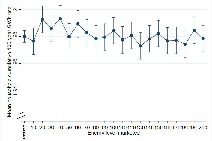
When testing if making households consider upgrading to a specific energy standard by marketing energy standards ranging from 10-200 \(kWh\)/(\(m^{2}a\)), no marketing of certain energy standards gives a statistically significant decrease in the mean 100-year cumulative heating energy need for households. Marketing of an energy standard of 20 and 40 \(kWh\)/(\(m^{2}a\)) gives a statistically significant increase in the mean 100-year cumulative heating energy need for households. Marketing of an energy standard of 10 \(kWh\)/(\(m^{2}a\)) gives a statistically significant improvement on the final energy standard. See Figure 2 for a visualization of the effect and Table 6 for the regression models.
| Model marketing-cumulative \(R^{2} = .05\), \(p < .00005\) \(N = 5000\) |
Model marketing-final \(R^{2} = .03\), \(p < .00005\) \(N = 5000\) |
|||
| Variable | Coef. (SE) | p | Coef. (SE) | p |
| Ambition marketed in \(kWh\)/(\(m^{2}a\)) | ||||
| 10 | -3448 (5488) | .530 | -1.78 (0.62)** | .004 |
| 20 | 12614 (5488)* | .022 | -1.06 (0.62) | .086 |
| 30 | 6030 (5488) | .272 | 1.04 (0.62) | .094 |
| 40 | 13095 (5488)* | .017 | 0.05 (0.62) | .938 |
| 50 | -256 (5488) | .963 | -0.21 (0.62) | .732 |
| 60 | 9370 (5488) | .088 | 0.47 (0.62) | .450 |
| 70 | 2664 (5488) | .627 | -0.73 (0.62) | .238 |
| 80 | -1599 (5488) | .771 | 0.21 (0.62) | .734 |
| 90 | -429 (5488) | .938 | -0.17 (0.62) | .787 |
| 100 | 4394 (5488) | .423 | 0.81 (0.62) | .188 |
| 110 | -2481 (5488) | .651 | -0.17 (0.62) | .778 |
| 120 | 776 (5488) | .887 | -0.26 (0.62) | .669 |
| 130 | -6916 (5488) | .208 | 0.64 (0.62) | .299 |
| 140 | -1598 (5488) | .771 | -0.23 (0.62) | .711 |
| 150 | 2161 (5488) | .694 | 0.89 (0.62) | .151 |
| 160 | -3167 (5488) | .564 | -0.11 (0.62) | .857 |
| 170 | -2821 (5488) | .607 | 0.12 (0.62) | .848 |
| 180 | -5707 (5488) | .298 | -0.08 (0.62) | .899 |
| 190 | 4742 (5488) | .388 | 1.17 (0.62) | .059 |
| 200 | -1486 (5488) | .786 | -0.08 (0.62) | .893 |
| Subsidies | ||||
| No subsidies | 31487.07** | \(<.00005\) | 2.30** | \(<.00005\) |
| Constant | 1964210 | \(<.00005\) | 131.30 | \(<.00005\) |
Policy 3: Motivating stage 3 households
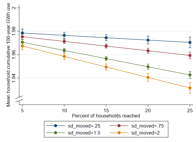
Giving households a “final push” to complete their retrofit by motivating households in stage 3 significantly affects both the mean 100-year cumulative heating energy need for households and the final energy standard, as long as both a broad outreach and significant changes to retrofit intention are achieved. See Figure 3 for a visualization of the effect and Table 7 for the regression models.
| Model push-cumulative \(R^{2} = .07\), \(p < .00005\) \(N = 9600\) |
Model push-final \(R^{2} = .03\), \(p < .00005\) \(N = 9600\) |
|||
| Variable | Coef. (SE) | p | Coef. (SE) | p |
| Percent of households reached | -202 (183) | .270 | -0.0114 (0.02) | .573 |
| SD move in intention | -2317 (2200) | .292 | 0.4046 (0.25) | .101 |
| Percent of households reached * SD move in intention | -796 (145)** | \(<.00005\) | -0.0621 (0.02)** | \(<.00005\) |
| Subsidies | ||||
| No subsidies | 28591 (1422)** | \(<.00005\) | 1.8565 (0.16)** | \(<.00005\) |
| Constant | 1966760 (2867) | \(< .00005\) | 131.81 (0.32) | \(< .00005\) |
Policy 4: Adjusting subsidy threshold
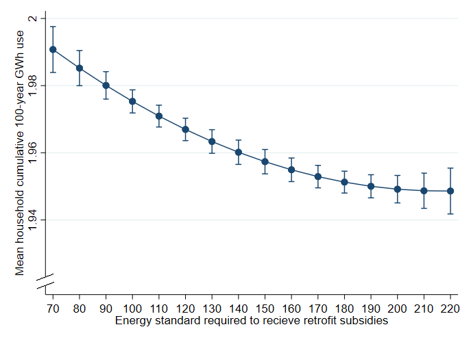
Adjusting the threshold for receiving policy support affects cumulative household energy use. Interestingly, making the threshold for receiving subsidies more ambitious leads to higher energy consumption on average because fewer households qualify for subsidies. Lowering the threshold to less ambitious retrofits with respect to the energy standard reduces energy consumption, but the effect has diminishing returns and reaches a floor at 210 \(kWh\)/(\(m^{2}a\)). Here, a further lowering of the required energy standard has no effect on more savings in the average energy use over 100 years. Although the curve tendency seems to indicate a slight increase after 210, all CI’s of the following points overlap with 210. Therefore, there is insufficient data to say that the curve is increasing. The real effect could be horizontal from 210 and out. No significant effect can be found on the final energy standard. See Figure 4 for a visualization of the effect and Table 8 for the regression models.
| Model adjusting-cumulative \(R^{2} = .03\), \(p < .00005\) \(N = 3100\) |
Model adjusting-final \(R^{2} = .01\), \(p < .00005\) \(N = 3100\) |
|||
| Variable | Coef. (SE) | p | Coef. (SE) | p |
| \(kWh\)/(\(m^{2}a\)) required | -847 (203)** | \(< .00005\) | -0.044 (0.24) | .062 |
| \(kWh\)/(\(m^{2}a\)) \(required^{2}\) | 1.95 (0.69)** | .005 | 0.00011 (0.0001) | .182 |
| Constant | 2040464 | \(<.00005\) | 135.1 | \(<.00005\) |
Discussion
Validity
Two out of three goals regarding the model’s validity were achieved, and the results of the policy simulations should be interpreted thereafter. Firstly, the only precisely replicated metric was the retrofitting rate. However, this metric was also used to parametrize the model, and only shows that repeated runs of the model give stable, similar results, represented by the low SD. As the model could not simulate findings regarding consecutive retrofitting, it should not be relied on regarding mechanisms surrounding households that undergo several retrofits. Because of this, the overall retrofit rate could be more equally distributed among households than in the real world. Likely, the model fails to capture “piecemeal retrofitting”, where homeowners first retrofit a wall, then a year later another wall, and two years later the ceiling. Future models could implement a more detailed representation of the technical standard of all parts of the households to possibly resolve this issue. Note that this would require further research on and altering the decision-making model. It must account for issues such as which parts of the house are retrofitted, if self-efficacy is part-specific, which motivational factors lead to upscaling the retrofit, and more.
Although some aspects of the model do not reflect reality, we argue the model still reflects a large enough portion of it to offer some interesting input to policy debates. Specifically, if a process happens without any involvement of piecemeal retrofitting, which it seems like the model does not capture, it should provide policy insight. In all scenarios where piecemeal retrofitting is a central part of the process, a higher level of care should be exerted when interpreting the results. The model should be helpful in exploring energy retrofit policymaking for private households that do not include piecemeal retrofitting. We discuss the results of the simulated policies below.
Policy scenarios
Policy 1: Current subsidy policy
According to the HERB model, the current Norwegian subsidy system reduces the 100-year heating need of an average household by 32934 \(kWh\), or 329 \(kWh\) a year. Although this number slightly drops when including policies 2 and 3 in the model, we argue this drop is so small that, in a practical sense, its impact on energy use is constant. The effects of the subsidy policy are not strengthened or weakened when policies 2 and 3 are implemented in the HERB model. In other words, the current energy subsidies reduce the energy consumption of Norwegian households, and this effect cannot be replaced by other policies in this article.
Additionally, it is worth noting that the difference in energy consumption between the policy and no policy scenarios is small. The no policy scenario (the constant in Table 1) consumed 1996420 \(kWh\), while the policy scenario consumed 1963486 \(kWh\). This is a reduction of 1.65%. In general, no policy in this paper was able to reduce energy consumption by more than 2-3%, suggesting policies could have a limited impact on the development of the building stock.
Policy 2: Marketing of specific energy standards
Concerning the suggested policy of marketing specific energy standards to the public, we can find no positive effect of marketing any energy standards. We find a negative effect of marketing a 20 and 40 \(kWh\)/(\(m^{2}a\)) standard. The rest of the marketed standards, from 10-200 \(kWh\)/(\(m^{2}a\)), have no statistically significant effect. There is likely a small negative effect of marketing energy standards between 40-80 \(kWh\)/(\(m^{2}a\)). If we had increased the number of simulations for each marketed standard to 500, we would most likely see a clearer trend here. But as the effect seems to be negative and small, establishing exactly how small this number is can be said to be unimportant. Note that this is tested with and without the current policy system testing in policy 1. In general, the effect marketing of specific energy standards is either non-existent or, more likely, too small to have any meaningful impact. Thus, we cannot suggest marketing any specific energy standard to the public as a policy for reducing the energy consumption of the housing stock.
In the model, the marketing of more ambitious energy standards most likely makes low-income households waste time considering upgrading to energy standards they can never afford, increasing the time it takes to upgrade to a realistic energy standard. Indeed, we see that generally, the average household cannot afford energy standards below 50 \(kWh\)/(\(m^{2}a\)).3 As worry about finances and financial gains are two of only three factors determining the transition from stage three, the cost of the retrofit is important for this stage. Possibly, households go faster through the lower stages with the promise of comfort but stop at the third and final stage, where finances matter more. Additionally, when several low-income households consider more ambitious energy standards, which will be a large expected increase in comfort, upgrading to a more realistic mid-end energy standard seems less appealing. Although some high-income households could benefit from considering a more ambitious energy standard and thus reach a low level of energy consumption faster, this seemingly does not compensate for its damaging effect on low-income households. While it in retrospect could seem obvious that marketing energy standards most people cannot afford did not work, it could have worked: Firstly, neighbours of the few households that went through with the upgrade would see their own energy standard as more wasteful. Second, when these households eventually deteriorate, other households could use their more realistic energy standards as an ambition.
On the other end, the marketing of a more realistic energy standard could slow the speed by which high-income households improve their energy standard. For example, say a household with an energy standard of 130 \(kWh\)/(\(m^{2}a\)) considers upgrading to a 50 \(kWh\)/(\(m^{2}a\)) energy standard that it actually would have completed given enough time. Then the marketing campaign convinces it to consider a 120 \(kWh\)/(\(m^{2}a\)) energy standard instead. Then the households will consider this standard for some time, not complete it as the financial and comfort gain is too small, which will ultimately increase the neighbourhood’s energy consumption.
According to the model, there seems to be no golden “middle road” where the marketed energy standard is low enough to make households retrofit to an energy standard they can afford and good enough so the energy saved is tangible. Although there could be aspects that the HERB model does not capture that make the marketing of certain energy standards a net positive for the building stock, the research and assumptions the model build on give no support for this policy.
Policy 3: Motivating stage 3 households
In contrast to the marketing approach, we find an effect of focusing policies towards motivating households at the «brink» of retrofitting. There is an interactive effect between the outreach of the policy and the motivational effect with no statistically significant main effects. This means that both variables have no impact on their own, but their impact relies on the other. The variables impact on energy consumption is outreach multiplied by effect, not outreach plus effect. Sufficient motivational measures or outreach will in itself have little to no effect. It should be noted that a general increase in intention to retrofit could be considered a method of overcoming the “there is never the right time” barrier, which is the largest barrier to retrofitting (Klöckner & Nayum 2016). Similar to policy 2, this policy is also tested with and without the current Norwegian policy system.
Note that outreach refers to the number of households that are already seriously considering retrofitting and not the population as a whole. Outreach campaigns can and should therefore be targeted. Because stage three primarily concerns financial aspects and some hopes for comfort, the campaigns should reflect this. Such measures could include free advisory services to help with budgeting and final planning problems (also suggested by Studer & Rieder 2019), contractor registers, and written testimonials from households that have already undergone retrofitting. It should be mentioned that in the real world, households generally view energy retrofitting positively (Haines & Mitchell 2014), most likely because of psychological mechanisms such as mere exposure (Zajonc 1968) and peak-end (Kahneman et al. 1993). Mere exposure is a psychological effect where the more a person is exposed to something, the more the person starts to like that thing. As retrofitting project usually takes some time, they will like the project more. Peak-end refers to the phenomenon where people evaluate events based on the most intense and the last emotion in an experience. Because at least the last emotion of a retrofit project, which is the completion, should be positive, the experience will be remembered more fondly than it actually was. Therefore, testimonials will generally be positive, and households advising against energy retrofitting themselves have completed should be rare.
The model does not specify how the household’s motivation is increased, only that it is. This leaves room for any measure that increases motivation. This could range from aspects that are in the model such as perceived gain in comfort, by advertising the increased thermal comfort in well-insulated households, or stem from original lines of research discovering new ways of motivating households that are seriously considering retrofitting. Therefore, the HERB model only states that the effect of the motivating measure, whatever it is, should ideally increase the motivation by above 1 SD and have an outreach of more than 15% of all stage 3 households. Note that 1 SD is quite a substantial increase in motivation and will require a well-designed campaign. For example, to achieve a 1 SD increase in motivation, an average homeowner with a better motivation than 50% of all other homeowners, must increase motivation to be better than 84% of homeowners.
In the model, the reasons why increasing households’ intention to retrofit decreases energy consumption is reasonably straightforward. By increasing the motivation of some households in stage 3, a need for household’s motivation from the other built-in variables in the model is lower. This causes more households to go through with their energy retrofit project, improve their energy standards, and lower their energy use, reducing the neighbourhood’s cumulative energy consumption.
Policy 4: Modification of subsidy threshold
Regarding increasing or lowering the ambition of the energy standard required to be eligible for subsidies, the model finds a curvilinear relation where the more ambitious the threshold, the larger the cumulative energy use. This might appear counter-intuitive as more ambitious standards should result in more energy-efficient buildings, but stricter standards also reduce the number of households eligible for subsidies. This relationship continues until the threshold for subsidy is at 210 \(kWh\)/(\(m^{2}a\)), from where on no further reduction of cumulative energy use can be observed, rather the contrary. Based on these results, a conclusion seems to be that the best balance between ambition level and number of energy retrofits subsidies can be achieved with relatively unambitious threshold levels. This is reflected in a higher amount of overall energy saved over the course of 100 years, not the final achieved energy standard after 100 years, which means that the less ambitious threshold sets more households on the path to energy efficiency earlier in the process.
Note that other effects the HERB model does not account for could also affect this relationship. For example, ENOVA states that the main purpose of their current subsidy model is to drive up demand for high-end retrofit measures. The increased demand will reduce prices due to larger production, and the subsidies will stop when the technology is competitive (Egner & Klöckner 2021), a sort of ‘trickle-down technology’. The HERB model does not capture this aspect. Additionally, it should be considered that a less ambitious threshold for receiving subsidies should result in increased costs for the policy, both in money distributed and resources needed for the processing of more applications.
In the model, the varying accessibility of subsidies has several effects. Firstly, reducing the ambition of the threshold gives more people access to the subsidies. Having access to subsidies then becomes the standard, and retrofitting without subsidies becomes the outlier. This makes retrofitting without subsidies less attractive, which hampers the transition between stages 1 to 3. This should both decrease the time households considers and completes upgrading to any standard less ambitious than the subsidy threshold. As most households can afford mid-end energy standards, not thinking about retrofitting to anything less ambitious is generally favourable.
Heightening the threshold for accessing subsidies has the opposite effect. The more ambitious the threshold, the fewer households have access to subsidies, reducing the negative impact of not having access to subsidies. Although access to subsidies will have a larger effect when households consider more ambitious retrofits, these are few and far between. Although attractive, more ambitious retrofits can often not be brought to completion due to financial constraints. Thus, although high-income households will more often retrofit to a more ambitious standard in this setting, this is not enough to counteract the increased energy demand of the effect of low and medium-income households’ reduced retrofit activity.
Further research and limitations
The HERB model shows that it is possible to strongly base behavioural decision making specific to certain behaviours in existing quantitative research. Doing so has both advantages and disadvantages. Firstly, we argue that the agents’ behaviour is closer to real energy retrofitting behaviour than other models. The agents base their decisions on the same factors that other research has found to influence energy retrofitting behaviour. Additionally, the agents are directly based on real household survey responses. This makes the agents resemble real households more than other systems. However, this comes at a cost. The model is considerably more chaotic with thousands of unique agents with stochastic behaviour. Consequently, analysis of the model with individual agent-level data is computationally challenging. Additionally, the modeller must often make assumptions to ‘fill the gap’ of where the research is unclear or incomplete. For example, in this project, the research did not cover how households pick the energy standard they consider upgrading to, which was an essential part of making the model work.
The inclusion of widely used energy metrics allowed the model to easily incorporate other research such as the price of energy retrofitting (Galvin 2010) and give specific estimates on how many \(kWh\) a policy will save per household. The disadvantage of this is that this number is highly uncertain, and giving such a precise estimate could give both the modellers and policymakers a false sense of security. However, we believe the benefits outweigh the negatives as long as these numbers are communicated with sufficient caveates.
Both studies that look deeper into and improve the model are possible. The model is fit to investigate many relations that are not reported in this paper, primarily because of researcher capacity and to keep the paper at an acceptable length. For example, the model is well suited to highlight the peculiar relationship between free-riding rates and the actual effect of a policy. A household that is free-riding does not imply the subsidy had no effect. Possibly the policy impacted neighbours, which may again impacted the free-riding house. The HERB model is in an excellent position to enlighten this relation. The model could also investigate which psychological aspect should be used when marketing retrofitting. Increasing the personal multipliers for some households can be a simple way to illustrate marketing. How much the price must go down on highly ambitious energy standards because more households are buying it, to make a meaningful impact on energy saving can be shown in the model with some work. The effect of neighbourhood density and economic composition is also readily available to be tested. Many more changes can be made to the existing policies, where all variables can be adjusted. For example, accepting a smaller percentwise increase in energy standard or coverage of a larger share of the retrofit cost, including a larger share than 100%. Policy scenarios where the subsidies are only accessible for specific groups, such as low-income households, households that have not retrofitted for 25 years, large or small households, or a combination of these can also be tested. While we for this paper wanted to focus on specific policies, the model allows for many hypotheses to be tested.
Several aspects of the model can also be improved, as several assumptions in the model are based on expert opinion. As mentioned earlier, the model could be expanded to consider how households retrofit only parts of the house. This could make the model account for piecemeal retrofitting. One of the more central assumptions of the model is how households pick energy standards to consider upgrading to. This mechanism could be researched and subsequently redesigned. A seasonal system where households are both more motivated to, but also hesitant towards undergoing extensive retrofits in winter could also be researched and implemented. A system where houses are built and abandoned could also be implemented. Possibly houses are abandoned if falling under a certain threshold, or city planning forces some houses to be removed. Finally, some smaller parts of the model could be expanded on. For example, how households recover their available capital for investing in household retrofitting and how the energy standard of households degenerate is simplified. Households’ investment potential does not increase when the energy standard, and thus the house’s value increases. Although some researchers indicate that the market is generally unwilling to finance energy retrofitting (Hill 2019), the models’ rendition is probably simplified compared to the real world. Similarly, the retrofit cost relies on 11 years old data (Galvin 2010) and could be updated. As these cost data affect the psychological values ‘worry enough finances’, and ‘financial gain’, and the potential cancellation of the retrofit process after stage 3, it is a central value in the model. Thus, an updated retrofit cost estimate could heavily influence the model.
Finally, the model does not account for several factors beyond behaviour relevant to energy retrofitting. Firstly, the model does not simulate market supply. What contractors and suppliers are available to provide is obviously relevant for the households ability to retrofit. This could be especially relevant for the marketing of certain energy standards, where focusing on one type of energy standard could reduce the same standard’s cost. With some work, supply could be integrated into the model (as done in Rosales-Carreón & García-Díaz 2015). Similarly, many other factors not accounted for in this model affect energy retrofitting behaviour. This model only tries to capture the intention of households. Factors such as weather, improvements in technology, legal changes, energy price, and more, will impact retrofitting behaviour. Other models have explored similar topics (for an overview, see Hesselink & Chappin 2019; Jager 2021). When designing policies, factors not included in this model must be accounted for. We only claim that according to the elements accounted for in this model, the following conclusions apply.
Conclusions
This paper presents an ABM that simulates household retrofitting in a neighbourhood. In a simulated neighbourhood where each household represents a unique respondent to a national survey, the model introduces a novel decision-making algorithm based on existing behavioural research regarding energy retrofitting. From there, we simulated different policy scenarios to estimate their predicted effect on household energy consumption for heating. The model had problems capturing the phenomenon of continuous retrofitting, which is likely caused by it not allowing for piecemeal retrofitting. Despite this, we deem it valid enough to offer valuable input on policy design as long as the scenario does not involve piecemeal retrofitting. Firstly, we find that the current subsidy system reduces overall household energy consumption and cannot be fully replaced by the other non-subsidy-based policies we implemented. Second, we find no positive effects of marketing a specific energy standard to all households. Third, we see a positive impact of encouraging households which have come far in the decision-making process to make the last step to retrofit, and find an interaction effect between outreach and impact, meaning that enough households (at least 15%) need to be pushed enough for this strategy to make a recognizable impact. Finally, the model suggests a curvilinear relationship between subsidy threshold and energy consumption, where it interestingly shows that the less ambitious the threshold for receiving subsidies, the lower the average household energy consumption up to 210 \(kWh\)/(\(m^{2}a\)). This counter-intuitive effect is likely caused by less ambitious thresholds for subsidies getting implemented by larger shares of the population early.
Relative to policymaking, this study suggests subsidizing energy retrofitting is positive and that the threshold should be kept reasonably low. Additionally, marketing specific energy standards seem to have little to no effect. Finally, motivational campaigns towards households at the ‘brink’ of retrofitting seem to have a positive effect as long as the motivational effect is strong and sufficient outreach. Although some policies reduced energy consumption, it is worth noting that all effects were small, suggesting that policies could have a limited impact on the building stock. As with all models, factors that the model does not capture most likely influence all policies mentioned above, and the model is not and should not be interpreted as the ultimate sandbox for policies. This includes but is not limited to supply, weather, energy price and more. Yet still, if a policy works in the HERB model, we argue it has a better chance of working in the real world than a policy that does not work. Overall, we see the model as something that could be a helpful tool in household energy retrofit policymaking.
Acknowledgments
We thank Dr. Ray Galvin for help with the mathematical explanation regarding the non-linear relationship between energy retrofitting and final energy standard; Dr. Erlend Andenæs for his feedback on the validity of the retrofit degradation formula; and Dr. Wander Jager for help with the development of the HERB model.Notes
10 NOK \(\approx\) 1 EUR↩︎
For example, a small 40 \(m^{2}\) house must reach 120+(1600/50) = 152 \(kWh\)/(\(m^{2}a\)) to be eligble for the 120 \(kWh\)/(\(m^{2}a\)) subsidy. A larger 400 \(m^{2}\) house must reach 120+(1600/400) = 124 \(kWh\)/(\(m^{2}a\)) to be eligble for the same subsidy.↩︎
Varies over time. Can be observed by running «ask turtles [set ambition 50 set retrofit_cost runresult retrofit_cost_formula] type "Mean investment potential:" print round mean [investment_potential] of turtles type "Mean retrofit cost:" print round mean [retrofit_cost] of turtles» at various times in the model.↩︎
Appendix
The ODD protocol of the model is available online here.

References
ALBERINI, A., Bigano, A., & Boeri, M. (2014). Looking for free riding: Energy efficiency incentives and Italian homeowners. Energy Efficiency, 7(4), 571–590. [doi:10.1007/s12053-013-9241-7]
BAMBERG, S. (2007). Is a stage model a useful approach to explain car drivers’ willingness to use public transportation? Journal of Applied Social Psychology, 37(8), 1757–1783. [doi:10.1111/j.1559-1816.2007.00236.x]
BAMBERG, S. (2013a). Applying the stage model of self-regulated behavioral change in a car use reduction intervention. Journal of Environmental Psychology, 33, 68–75. [doi:10.1016/j.jenvp.2012.10.001]
BAMBERG, S. (2013b). Changing environmentally harmful behaviors: A stage model of self-regulated behavioral change. Journal of Environmental Psychology, 34, 151–159. [doi:10.1016/j.jenvp.2013.01.002]
BORIA, E. S. (2020a). Investing in the future by encouraging energy retrofit decisions. University of Illinois at Chicago, PhD Thesis. Available at: https://indigo.uic.edu/articles/thesis/Investing_in_the_Future_by_Encouraging_Energy_Retrofit_Decisions/13475115.
BORIA, E. S. (2020b). Neighbor influenced energy retrofit (NIER) agent-Based model. v1.0.0, CoMSES Computational Model Library. Available at: https://www.comses.net/codebases/e0f12da8-a9d0-48a1-9446-30275482a8b4/releases/1.0.0/.
COLLINS, M., & Curtis, J. (2018). Willingness-to-pay and free-riding in a national energy efficiency retrofit grant scheme. Energy Policy, 118, 211–220. [doi:10.1016/j.enpol.2018.03.057]
EGNER, L. E., & Klöckner, C. A. (2021). Temporal spillover of private housing energy retrofitting: Distribution of home energy retrofits and implications for subsidy policies. Energy Policy, 157, 112451. [doi:10.1016/j.enpol.2021.112451]
EGNER, L. E., Klöckner, C. A., & Masini, G. P. (2021). Low free-riding at the cost of subsidizing the rich. Replicating Swiss energy retrofit subsidy findings in Norway. Energy and Buildings, 253, 111542. [doi:10.1016/j.enbuild.2021.111542]
ELEFTHERIADIS, G., & Hamdy, M. (2017). Impact of building envelope and mechanical component degradation on the whole building performance: A review paper. Energy Procedia, 132, 321–326. [doi:10.1016/j.egypro.2017.09.739]
ENOVA. (2019). Beskrivelse av tekniske kriterier ved tilskudd til oppgradering av bolig. Available at: https://www.enova.no/privat/alle-energitiltak/oppgradere-huset/oppgradering-av-bygningskroppen-/.
EUROPEAN Commission. (2020). A renovation wave for Europe - Greening our buildings, creating jobs, improving lives. Available at: https://eur-lex.europa.eu/legal-content/EN/TXT/?uri=COM:2020:0662:FIN.
EUROSTAT. (2019). Energy consumption in households. Available at: https://ec.europa.eu/eurostat/statistics-explained/index.php/Energy_consumption_in_households.
FEDERAL Office for the Environment. (2018). Swiss climate policy. Available at: https://www.bafu.admin.ch/bafu/en/home/topics/climate/info-specialists/climate-policy.html.
FRIEGE, J., Holtz, G., & Chappin, E. J. L. (2016). Exploring homeowners’ insulation activity. Journal of Artificial Societies and Social Simulation, 19(1), 4: https://www.jasss.org/19/1/4.html. [doi:10.18564/jasss.2941]
FYHN, H., Berntsen, A., Egner, L. E., Johansen, J. P. K., Klöckner, C. A., Nilsen, B. T., Nilsen, M., & Røyrvik, J. O. D. (2019). Evaluering av Enovas satsing på oppgradering av eksisterende boliger. Available at: https://ntnuopen.ntnu.no/ntnu-xmlui/handle/11250/2610979.
GALVIN, R. (2010). Thermal upgrades of existing homes in Germany: The building code, subsidies, and economic efficiency. Energy and Buildings, 42(6), 834–844. [doi:10.1016/j.enbuild.2009.12.004]
GALVIN, R., & Sunikka-Blank, M. (2013). Economic viability in thermal retrofit policies: Learning from ten years of experience in Germany. Energy Policy, 54, 343–351. [doi:10.1016/j.enpol.2012.11.044]
GILLARD, R., Snell, C., & Bevan, M. (2017). Advancing an energy justice perspective of fuel poverty: Household vulnerability and domestic retrofit policy in the United Kingdom. Energy Research & Social Science, 29, 53–61. [doi:10.1016/j.erss.2017.05.012]
GRIMM, V., Berger, U., Bastiansen, F., Eliassen, S., Ginot, V., Giske, J., Goss-Custard, J., Grand, T., Heinz, S. K., Huse, G., Huth, A., Jepsen, J. U., JNørgensen, C., Mooij, W. M., Müller, B., Pe’er, G., Piou, C., Railsback, S. F., Robbins, A. M., … DeAngelis, D. L. (2006). A standard protocol for describing individual-based and agent-based models. Ecological Modelling, 198(1), 115–126. [doi:10.1016/j.ecolmodel.2006.04.023]
GRÖSCHE, P., Schmidt, C. M., & Vance, C. (2009). Identifying free-riding in energy-Conservation programs using revealed preference data. Available at: https://papers.ssrn.com/sol3/papers.cfm?abstract_id=1375365.
HAINES, V., & Mitchell, V. (2014). A persona-based approach to domestic energy retrofit. Building Research and Information, 42(4), 462–476. [doi:10.1080/09613218.2014.893161]
HAUGLAND, T. (1996). Social benefits of financial investment support in energy conservation policy. Energy Journal, 17(2). [doi:10.5547/issn0195-6574-ej-vol17-no2-5]
HELMS, A. C. (2012). Keeping up with the Joneses: Neighborhood effects in housing renovation. Regional Science and Urban Economics, 42(1–2), 303–313. [doi:10.1016/j.regsciurbeco.2011.07.005]
HESSELINK, L. X. W., & Chappin, E. J. L. (2019). Adoption of energy efficient technologies by households – Barriers, policies and agent-based modelling studies. Renewable and Sustainable Energy Reviews, 99, 29–41. [doi:10.1016/j.rser.2018.09.031]
HILL, D. R. (2019). Energy efficiency financing: A review of risks and uncertainties. 42nd IAEE International Conference, Montreal, Canada.
JAGER, W. (2021). Using agent-based modelling to explore behavioural dynamics affecting our climate. Current Opinion in Psychology, 42, 133–139. [doi:10.1016/j.copsyc.2021.06.024]
KAHNEMAN, D., Fredrickson, B. L., Schreiber, C. A., & Redelmeier, D. A. (1993). When more pain is preferred to less: Adding a better end. Psychological Science, 4(6), 401–405. [doi:10.1111/j.1467-9280.1993.tb00589.x]
KERR, N., & Winskel, M. (2020). Household investment in home energy retrofit: A review of the evidence on effective public policy design for privately owned homes. Renewable and Sustainable Energy Reviews, 123, 109778. [doi:10.1016/j.rser.2020.109778]
KLÖCKNER, C. A., & Nayum, A. (2016). Specific barriers and drivers in different stages of decision-Making about energy efficiency upgrades in private homes. Frontiers in Psychology, 7, 1362.
LEE, J. S., Filatova, T., Ligmann-Zielinska, A., Hassani-Mahmooei, B., Stonedahl, F., Lorscheid, I., Voinov, A., Polhill, G., Sun, Z., & Parker, D. C. (2015). The complexities of agent-based modeling output analysis. Journal of Artificial Societies and Social Simulation, 18(4), 4: https://www.jasss.org/18/4/4.html. [doi:10.18564/jasss.2897]
LIANG, X., Yu, T., Hong, J., & Shen, G. Q. (2019). Making incentive policies more effective: An agent-based model for energy-efficiency retrofit in China. Energy Policy, 126, 177–189. [doi:10.1016/j.enpol.2018.11.029]
NAIR, G., Gustavsson, L., & Mahapatra, K. (2010). Owners perception on the adoption of building envelope energy efficiency measures in Swedish detached houses. Applied Energy, 87(7), 2411–2419. [doi:10.1016/j.apenergy.2010.02.004]
NAULEAU, M. L. (2014). Free-riding on tax credits for home insulation in France: An econometric assessment using panel data. Energy Economics, 46, 78–92. [doi:10.1016/j.eneco.2014.08.011]
OTTE, G. (2008). Sozialstrukturanalysen mit Lebensstilen. Berlin Heidelberg: Springer.
PALMER, K., Walls, M., & Gerarden, T. (2012). Borrowing to save energy: An assessment of energy-efficiency financing programs. Available at: https://www.rff.org/publications/reports/borrowing-to-save-energy-an-assessment-of-energy-efficiency-financing-programs/. [doi:10.1007/s12053-012-9178-2]
POLHILL, J. G., Parker, D., Brown, D., & Grimm, V. (2008). Using the ODD protocol for describing three agent-based social simulation models of land-use change. Journal of Artificial Societies and Social Simulation, 11(2), 3: https://www.jasss.org/11/2/3.html. [doi:10.18564/jasss.1563]
RIVERS, N., & Shiell, L. (2016). Free-Riding on energy efficiency subsidies: The case of natural gas furnaces in Canada. The Energy Journal, 37(4). [doi:10.5547/01956574.37.4.nriv]
ROSALES-CARREÓN, J., & García-Díaz, C. (2015). Exploring transitions towards sustainable construction: The case of near-zero energy buildings in the Netherlands. Journal of Artificial Societies and Social Simulation, 18(1), 10: https://www.jasss.org/18/1/10.html.
SSB. (2019). 09587: Innenlandske flyttinger, etter flytteregion, kjønn og alder 2005 - 2020. Available at: https://www.ssb.no/statbank/table/09587.
SSB. (2021a). e01222: Endringar i befolkninga i løpet av kvartalet, for kommunar, fylke og heile landet. Available at: https://www.ssb.no/statbank/table/01222.
SSB. (2021b). Forsinket befolkningsstatistikk på rutenett [Data set]. In Forsinket befolkningsstatistikk på rutenett. Available at: https://kart.ssb.no/.
STUDER, S., & Rieder, S. (2019). What can policy-Makers do to increase the effectiveness of building renovation subsidies? Climate, 7(2), 28. [doi:10.3390/cli7020028]
TVERSKY, A., & Kahneman, D. (1973). Availability: A heuristic for judging frequency and probability. Cognitive Psychology, 5(2), 207–232. [doi:10.1016/0010-0285(73)90033-9]
UNITED Nations - UN. (1987). Report of the World Commission on Environment and Development: Our common future. Available at: http://www.ask-force.org/web/Sustainability/Brundtland-Our-Common-Future-1987-2008.pdf
VERBEECK, G., & Hens, H. (2005). Energy savings in retrofitted dwellings: Economically viable? Energy and Buildings, 37(7), 747–754. [doi:10.1016/j.enbuild.2004.10.003]
WATTS, D. J., & Strogatz, S. H. (1998). Collective dynamics of small-world networks. Nature, 393(6684), 440–442. [doi:10.1038/30918]
WILSON, C., Boe, B., Sala, A., Puttaswamy, K. P. N., & Zhao, B. Y. (2009). User interactions in social networks and their implications. Proceedings of the Fourth ACM European Conference on Computer Systems - EuroSys’09,Nuremberg, Germany. [doi:10.1145/1519065.1519089]
ZAJONC, R. B. (1968). Attitudinal effects of mere exposure. Journal of Personality and Social Psychology, 9(2), 1–27. [doi:10.1037/h0025848]