Luis R. Izquierdo and J. Gary Polhill (2006)

Is Your Model Susceptible to Floating-Point Errors?

Journal of Artificial Societies and Social Simulation vol. 9, no. 4
<https://www.jasss.org/9/4/4.html>

For information about citing this article, click here

Received: 18-Jan-2006    Accepted: 12-Oct-2006    Published: 31-Oct-2006

Abstract

This paper provides a framework that highlights the features of computer models that make them especially vulnerable to floating-point errors, and suggests ways in which the impact of such errors can be mitigated. We focus on small floating-point errors because these are most likely to occur, whilst still potentially having a major influence on the outcome of the model. The significance of small floating-point errors in computer models can often be reduced by applying a range of different techniques to different parts of the code. Which technique is most appropriate depends on the specifics of the particular numerical situation under investigation. We illustrate the framework by applying it to six example agent-based models in the literature.

Keywords:

Floating Point Arithmetic, Floating Point Errors, Agent Based Modelling, Computer Modelling, Replication

Introduction

1.1

If a model uses floating-point numbers, chances are that it is suffering floating-point errors. However, the important question is not whether there are floating-point errors in the model (which there almost certainly are); neither is it whether these errors occur frequently. The question is not even (necessarily) whether the results obtained from the model are significantly affected by floating-point errors. The key question is whether floating-point errors have a substantial impact on whatever the model is used for. In short, the model might be suffering floating-point errors, but … does it really matter?

1.2

It is clear that there cannot be a general answer for such a question. The answer not only depends on the particular model under consideration but also, and crucially, on the specific use the researcher makes of it. Since researchers use models for very different purposes, in order to assess whether floating-point errors are something to worry about or not, the best that can be provided is a framework that assists researchers in finding out the answer for themselves in any specific case they might encounter. The aim of this paper is to provide such a framework. We use six agent-based models that have formed the basis of several scientific publications to illustrate both the use and the usefulness of the framework. These models are:

1. Axelrod's model of metanorms (Axelrod 1986; Galán & Izquierdo 2005).
2. The Artificial Stock Market, or ASM (LeBaron et al. 1999; Johnson 2002).
3. FEARLUS (Polhill et al. 2001; Gotts et al. 2003).
4. BM (Macy & Flache 2002; Flache & Macy 2002).
5. CASD (Izquierdo et al. 2004)
6. CharityWorld (Polhill et al. 2006).

1.3

More specifically, the framework provided here is aimed at assisting the reader in identifying whether a particular model might behave significantly differently when run in a floating-point environment versus when run following the rules of real arithmetic. The rationale for studying such a question derives from the observation that many modellers readily assume that their floating-point model is behaving as if it was running under real arithmetic. Thus, in broader terms, this paper is about the extent to which a particular simulation model is an accurate representation of the modeller's intentions or specifications; significant differences in behaviour using the two arithmetic systems most often imply significant differences between what the modeller believes is happening in a model and what is actually happening.

1.4

In this paper, we regard the behaviour of the model in real arithmetic as the correct one because the use of real arithmetic ensures the prevalence of several laws (e.g. the associative law of addition, the associative law of multiplication, and the distributive law between multiplication and addition) which are usually considered desirable in modelling real-world systems, and which do not necessarily hold in floating-point arithmetic. This, in turn, is one of the reasons why most modellers' intent is to run their simulations using real arithmetic.

1.5

The relevance of floating-point errors in computer modelling has already been demonstrated by Polhill et al. (2005), who showed how two well known agent-based models can be substantially affected by these errors (also, see another striking illustration of the importance of floating-point errors in computer models in Appendix B). Following that work, Polhill et al. (2006) conducted a thorough evaluation of a wide range of techniques that can be used to mitigate the impact of floating-point errors, with interval arithmetic being identified as the most promising way forward. However, given the advanced level of programming expertise required to put into practice some of the measures proposed by Polhill et al. (2006), it is conceivable that not many computer modellers will actually implement them, particularly if they are not convinced that floating-point errors are an issue in their models. This paper aims to facilitate the task of finding out whether a model is significantly affected by floating-point errors and, if so, whether it really matters. This is done by providing a framework that (a) highlights the features of models that make them especially vulnerable to floating-point errors and (b) suggests ways in which floating-point problems can be avoided or mitigated to some extent.

The very basics of floating-point arithmetic

2.1

Many of the calculations implemented in formal models involve numbers that are not necessarily integers. When these calculations take place in a computer, the standard way of conducting them is using floating-point arithmetic. The use of floating-point numbers derives from the requirement of working with an infinite and fully connected set of numbers (e.g. the real numbers) in a machine that can only employ a finite bit string to represent that set. Polhill et al. (2006) provide a brief introduction to how floating-point numbers work; Goldberg (1991) and Higham (2002, ch. 1 and 2) give more advanced and extensive introductions to the topic. Roughly speaking, within a very wide range, the floating-point representation of a number x consists of the n most significant digits of x in a base b (i.e. the number x written in scientific notation in base b)^[1]. For instance, the closest floating-point number to 7654321 in a decimal floating-point system with 4 digits of precision would be 7.654·10⁶. Thus, floating-point systems have the convenient property that the density of representable numbers in a range is related to the magnitude of the numbers in that range (i.e. representable numbers are not equally spaced): the smaller the magnitude of the numbers in a range, the higher the density of floating-point numbers in that range (Figure 1). As an example, using the types float or double in C, roughly half of all representable floating-point numbers are between –1 and 1.

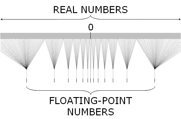
Figure 1. Schematic illustration of the correspondence between the set of real numbers and their floating-point representation in a computer. The set of real numbers is fully connected and unbounded, whereas the set of floating-point numbers in a computer is sparse and bounded

2.2

Whilst inexact by nature, floating-point numbers in most computers are impressively accurate. To measure their accuracy, numerical analysts define the unit roundoff u, which is the maximum relative error in approximating any real number (within the range of the floating-point system) by its closest representable floating-point number. The unit roundoff in double precision IEEE 754 standard floating-point numbers (IEEE 1985) is 2^–53 ≈ 1·10^–16, and the range is approximately [10^–308, 10⁺³⁰⁸]. Thus, double precision IEEE floating-point numbers give between 15-17 significant decimal digits of accuracy. Since floating-point systems in most modern processors and platforms follow the IEEE 754 standard, the following discussion will focus on this standard.

2.3

IEEE floating-point arithmetic is also impressively precise. The standard stipulates that (in the default rounding mode) all arithmetic operations (+, –, ×, /) should be computed as though the precision is infinite and the result is rounded to the nearest representable number. This is termed exact rounding (Goldberg 1991). Exact rounding, however, does not guarantee that the relative error after a small number of sequential calculations will be necessarily small. Higham (2002, p. 9) provides some striking (though admittedly extreme) examples where the relative error can be as high as 50% after just four simple operations. Note also that exact rounding refers to operations with floating-point numbers, not with real numbers – e.g. (0.3 / 0.1) does not equal 3 in IEEE double precision arithmetic.

2.4

What is essential to realise is that if a model uses floating-point numbers, then it is almost certain that it will suffer floating-point errors. This is so for two reasons:

1. The set of floating-point numbers is discrete and bounded, whereas the set of real numbers is continuous and unbounded. Figure 1 sketches this many(actually infinite)-to-one function that relates real numbers with their floating-point representation. Thus, most real numbers are not exactly representable in the floating-point systems used in computers.
2. Most modern computers use base 2 in their floating-point number system (Higham 2002, p. 47). This means that any number which is not exactly representable in base 2 will have some rounding error. In particular, most base 10 decimal fractions will have rounding errors. As an example, in single or double precision IEEE 754, only 63 of the 999999 numbers of the form 0.000001·i (i = 1, 2… 999999) are exactly representable.

Scope of this paper

3.1

While acknowledging that floating-point errors can accumulate to a large extent in some models, this paper focuses on the impact of small errors. There are three reasons for this:

1. As explained above, it is almost certain that every model that uses floating-point numbers suffers floating-point errors. However, there is no reason to believe that these errors accumulate to a large extent in general.
2. Small errors can have major impacts. Even when errors do not accumulate to a large extent, the results of a model can be potentially meaningless due to very small floating-point errors. The main reason for this is that, when models have branching statements, even the smallest error can make the model follow the wrong branch, and the consequences of deviating from the right path are potentially enormous.
3. The problems caused by small errors are also present when errors accumulate, so all the issues addressed in this paper are also relevant for models with large errors.

3.2

Though the three points above argue for the usefulness of this paper, they also reveal a disturbing fact: in the best possible scenario, the framework provided here will assist in determining that floating-point errors do not significantly affect any conclusions provided errors do not accumulate to a large extent. Unfortunately, there is not a simple rule to avoid accumulation of floating-point errors. In fact, such a task is sometimes impossible and, even when possible, it is by no means trivial even for experienced numerical analysts. The silver lining is that by investigating the potential impact of small errors in a (sufficiently simple) model, it is likely that we will be able to acquire a reasonable idea of the extent to which errors accumulate.

The heart of the framework: Knife-edge thresholds

4.1

As mentioned above, one of the main problems we face when using floating-point numbers in a model is that (a) floating-point errors will almost certainly occur, and (b) even the smallest floating-point error can make the model follow the wrong path. This means that the difference between the correct result and the computed one is potentially massive even if errors do not accumulate since, quite simply, the model may not be conducting the operations it should. The problem of performing the wrong operations due to floating-point errors is created by what we call knife-edge thresholds. Knife-edge thresholds are branching statements^[2] (e.g. IF(condition)–THEN(action)) where the condition part involves a comparison with a floating-point number, and the subsequent action(s) create some kind of discontinuity. As an example, consider the following program, which, using IEEE 754 standard double precision, results in the undue death of an agent:

ENERGY = 0.6; ENERGY = ENERGY – 0.2; ENERGY = ENERGY – 0.4; IF (ENERGY < 0) THEN (AGENT DIES);

4.2

Whether or not the undue death of an agent significantly affects any conclusions based on the model is something that will depend on the type of conclusions being drawn from the model, which is why a framework rather than a more rigorous methodology is the best that can be provided.

Overview of the framework

5.1

The framework consists of a series of actions and recommendations that are intended to assist the reader in assessing whether the conclusions obtained with a model may be affected by floating-point errors. For the benefit of the reader, Figure 2 presents the framework as a step-wise methodology. However, we would rather describe our work as a framework for various reasons:

1. Advanced users can sometimes skip various steps in the methodology, since just one or a few steps often suffice to appropriately deal with floating-point issues (which steps are most useful depends on each particular case).
2. There is often more than one step in the methodology that can be applied to solve a specific floating-point problem, and the one that comes first in the step-wise methodology is not always necessarily the easiest to implement.
3. Undertaking certain actions in the list can enhance the usefulness of previous steps, so it is often useful to iterate through the step-wise methodology.

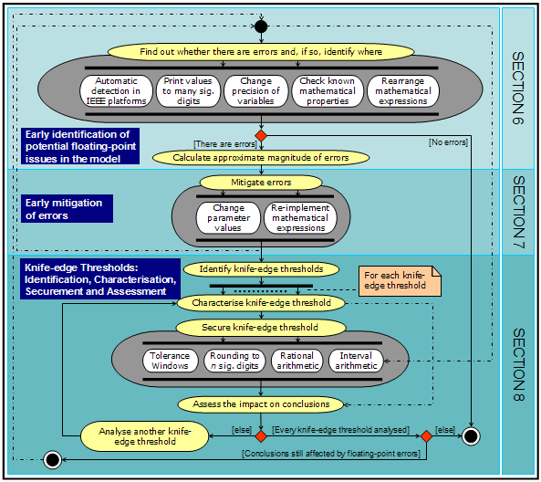
Figure 2. UML Activity diagram (Booch et al. 1999) of a step-wise methodology to deal with floating-point errors in a model. This methodology is not meant to be prescriptive; it is offered only as a guideline. Many possible variants are possible, some of which are indicated using dotted-dashed arrows. White boxes contained in one single grey box denote actions aimed at achieving one common goal; there is not a fixed execution order for these, and just a few of them may be sufficient to achieve the goal

5.2

The first proposed action is to become familiar with potential floating-point issues in the model. This requires finding out whether errors are occurring at all and, if so, identifying where they are occurring and calculating the approximate magnitude of the error. Several guidelines on how to do this are given in section 6.

5.3

Section 7 explains two sets of simple actions aimed at mitigating the impact of floating-point errors. These actions can be undertaken before conducting a thorough study of every knife-edge threshold in the model, and they will potentially facilitate the analysis to a great extent.

5.4

Section 8 is the core part of the framework. It explains how to identify knife-edge thresholds (identification; section 8.1), what features should be considered to deal with them appropriately (characterisation; section 8.2), what techniques can be applied to make sure that the correct branch is always selected (securement; section 8.3), and how to assess their impact when they cannot be successfully secured (assessment; section 8.4).

Early identification of potential floating-point issues in the model

Error identification

6.1

The first question that needs to be answered is whether the model under investigation is suffering floating-point errors at all. In general, it will be necessary to identify all the floating-point variables in the model (e.g. by using the Unix command grep) and then assess whether there is any chance that such variables will be meant to store values that they cannot store precisely (e.g. fractions which are not exactly representable in binary with a finite number of bits, like 0.1). The following techniques can assist in conducting such a task:

• If using a platform that fully complies with the IEEE 754 standard (e.g. C, C++, and Objective-C, but not Java at present), it is possible to conduct an automatic detection of floating-point errors at run-time; elsewhere (Polhill and Izquierdo 2005) we explain how to do this automatic check.
• Run the model and print the value of floating-point variables to many digits. For instance, printing the variable ENERGY to 30 significant digits after each of the first three statements in the piece of code introduced in section 0 gives the following output:

  ENERGY= 0.599999999999999977795539507497 ENERGY= 0.399999999999999966693309261245 ENERGY= -5.55111512312578270211815834045e-17

• Study the behaviour of the model after changing the precision of certain variables (e.g. replace floats with doubles, or vice versa).
• Check mathematical properties of the model that are known to hold in real arithmetic (e.g. stability of values that should remain constant throughout the simulation, like the number of shares in the ASM (Polhill and Izquierdo, 2005) or the total wealth in CharityWorld (Polhill et al. 2006)).
• Investigate the consequences of rearranging expressions in ways that are mathematically equivalent but numerically different (Polhill et al. 2005). For instance, replace a · (b + c) with a·b + a·c.

Early estimation of the magnitude of errors

6.2

To acquire an approximate idea of the magnitude of the error that may occur in a computation, we provide here a few well-known results on the precision of arithmetic operations (+, –, ×, /). What follows is valid for most computers (Higham 2002) and, in particular, holds for IEEE 754 standard arithmetic.

6.3

Arithmetic operations with floating-point operands (and also the square root in IEEE 754 standard arithmetic) are computed as though the precision is infinite and the result is rounded to the nearest representable number. This means that the relative error in the computed value of any valid arithmetic operation with floating-point operands is no greater than the unit roundoff u, which is approximately equal to 6·10^–8 in IEEE 754 standard single precision and 1·10^–16 in double precision. Mathematically,

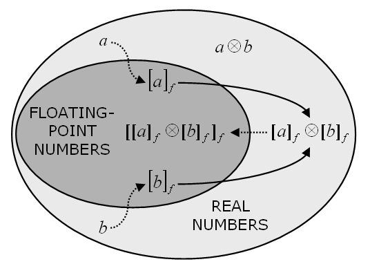
[ x ⊗ y ]f = ( x ⊗ y ) ·(1 + δ)

|δ| ≤ u

where x and y are two floating point numbers, [z]_f denotes the closest representable number to z, ⊗ stands for any arithmetic operation, and δ is the relative error. Note, however, that when performing an arithmetic operation (a ⊗ b) with real numbers a and b in a computer, the result is generally [[a]_f ⊗ [b]_f]_f , which may not coincide with [a ⊗ b]_f. This potential discrepancy, illustrated in Figure 3, explains why (0.3 / 0.1) does not equal 3 in IEEE 754 double precision arithmetic, even though [3]_f ≡ 3.

Figure 3. Schematic representation of stages in a floating-point calculation with two real operands a and b to the floating-point result [[a]f ⊗ [b]f]f. Dotted lines show conversion from a non-representable to a representable number, and hence a potential source of error, whilst the solid lines indicate the operation

6.4

When summing n floating-point numbers {x_i}, assuming that no number x_i takes part in more than n–1 additions^[3], Higham (2002) shows that the final result is the exact sum of terms x_i·(1 + ε_i) with |ε_i| ≤ (nu / (1 – nu)). In particular, if all summands have the same sign, then the relative error of the final result is at most nu.

6.5

As for multiplication and division, it is worth saying that while over the whole set of floating-point numbers there are just as many exact divisions as there are exact multiplications (ignoring the number 0 as an operand), such equivalence does not hold within subsets of representable numbers. For instance, division between members of the set of representable integers is much more likely to give errors than multiplication (e.g. while every multiplication between integers in the range [1, 10000] is exact, less than 0.5% of the divisions are).

6.6

From now on, we assume that the model under investigation does suffer floating-point errors. The following section outlines two sets of (preliminary) actions that could mitigate the effect of these errors: changing the parameter values, and re-arranging mathematical expressions.

Early mitigation of errors

Early mitigation of errors by changing parameter values

7.1

There are several computer models which, if run according to the laws of real arithmetic, would exhibit the same behaviour for different parameterisations as long as certain relations between their parameters are satisfied. This property is often lost in the realm of floating-point arithmetic, where some of those parameterisations will cause more errors than others (see a striking illustration of this in Appendix B). This is the case in Axelrod's model of metanorms (henceforth RAEAN^[4]), CASD, BM, and CharityWorld.

7.2

In RAEAN, CASD, and BM, the agents in the model make decisions (e.g. to cooperate or to defect) and then they receive a certain payoff which is calculated according to a specified payoff matrix. In real arithmetic, the behaviour of the three models is invariant to multiplications of the payoff matrix by a constant^[5] (this is often the case in game-theoretical models). In floating-point arithmetic, however, results can be different. This is illustrated in Figure 4, which shows two runs conducted with RAEAN that should exhibit exactly the same behaviour, but whose outputs are radically different. In one of the runs (hereafter the 'baseline run') all the payoffs are integers; in the other run, every payoff has been divided by 10 to produce a non-representable decimal fraction. An additional control run where all the payoffs used in the baseline run were multiplied by 10 gave exactly the same results as the baseline run.

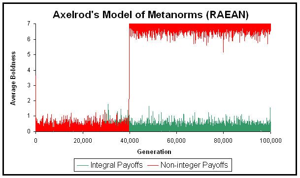
Figure 4. Population average boldness in two sample runs conducted with RAEAN. The two runs differ only in the magnitude of the payoffs. The green line shows a run in which all the payoffs are integers (T = 3; H = –1; E = –2; P = –9; ME = –2; MP = –9), while the red line shows a run in which all the payoffs have been divided by 10 (T = 0.3; H = –0.1; E = –0.2; P = –0.9; ME = –0.2; MP = –0.9). In real arithmetic, the two runs should give exactly the same output. The program and all the parameters used in this experiment are available in the Supporting Material

7.3

Figure 4 does not show a special case. Out of 1000 pairs of simulations where each member of the pair should exhibit exactly the same behaviour (using the same parameters as in Figure 4, but a different random seed for each pair), in 999 cases the simulation results differed. We also ran 1000 additional control runs where the baseline integral payoffs used in Figure 4 were multiplied by 10, and no differences were found in any of these 1000 pairs. Thus, it seems clear that the runs with integral payoffs suffered fewer floating-point errors than the runs conducted with non-integral payoffs. It is worth mentioning that using IEEE 754 double precision, every addition, subtraction, or multiplication using integers in the range [–94906266, 94906266] is exact.

7.4

If only integral payoffs are used in CASD, the model behaves exactly as with real arithmetic. Similarly, virtually every version of CharityWorld behaves as with real arithmetic if appropriate care is taken in choosing the parameters (see Polhill et al. 2006).

7.5

Thus, a clear recommendation is, if possible, to use parameter values that minimise the chances of getting floating-point errors. In particular, when exploring the parameter space of a model, it is advisable to sample parameter values that have few digits in binary^[6] rather than simple-looking numbers in base 10. For instance, select multiples of 9.765625·10^–4 rather than multiples of 0.001. In double precision, the closest representable number to 0.001, i.e. [0.001]_f , has 51 significant bits out of the 53 bits of accuracy that the format stipulates; on the other hand, 9.765625⋅10^–4, which is exactly representable, has only one significant bit.

[0.001]_f is stored (in binary) as:
1.0000011000100100110111010010111100011010100111111100 · 2^–10

9.765625·10^–4 ≡ [9.765625·10^–4]_f is stored as:
1.0000000000000000000000000000000000000000000000000000 · 2^–10

7.6

Thus, the chances of getting an inexact result are higher when using [0.001]_f as an operand, rather than [9.765625·10^–4]_f. The same applies for models that use empirical data: values should be rounded to exactly representable base 2 numbers, instead of simple-looking base 10 numbers. Our experience is that inputting numbers that are not exactly representable is very often the reason behind the appearance of the first floating-point error in a model. On the other hand, when dealing with representable numbers with few bits (e.g. small integers), it is often not until a division takes place that the first floating-point error appears.

Early mitigation of errors by re-implementing mathematical expressions

7.7

Expressions that are equivalent in real arithmetic may not be equivalent numerically (see a striking illustration of this in Appendix B): much effort in the field of numerical analysis is devoted to the study of the accuracy and stability of different algorithms that are equivalent in real arithmetic. Obviously, this paper is by no means a substitute for that, and the interested reader should refer to the vast literature in numerical analysis. Higham (2002) provides an excellent introduction to the topic, and gives recommendations for common operations like summation (pp. 89–90). Chan et al. (1983) offer recommendations on computing the sample variance, an operation which is commonly performed in computer models (e.g. RAEAN and the ASM). Whenever it is possible to pass twice through the data, Chan et al. (1983) recommend using the following formula to compute the sum of squares of the deviations from the mean in a set of N data points {x_i}:

7.8

In general, one can sometimes avoid the appearance of errors by rearranging expressions in fairly trivial ways. As an example, consider the following condition, which is used in Axelrod's model of metanorms (Axelrod 1986, p. 1099) to check whether one particular number x_j in a set of N data points {x_i} exceeds the average of the set by at least one standard deviation σ:

(1)

7.9

This condition would be naturally implemented as:

(1a)

7.10

Implementation [1a] will almost certainly suffer from floating-point errors because of the divisions and the square root. However, assuming that {x_i} are integers, and {x_i} and N are not too large^[7] (both conditions prevail in Axelrod's paper), the following rearrangement will prevent any errors from happening^[8]:

(1b)

7.11

Similar examples can be found in CharityWorld, where

(2a)

should be substituted by

(2b)

if {x_i} are integers.

Knife-edge Thresholds: Identification, Characterisation, Securement and Assessment

Identification of knife-edge thresholds

8.1

Potential knife-edge thresholds can be identified conducting an automatic search for comparison operators. However, note that not every branching statement with a comparison involving a floating-point variable is a knife-edge threshold. For example, the following implementation of the absolute value of a floating-point number is not a knife-edge threshold, since there are no discontinuities in the algorithm.

IF (x < 0.0) THEN (x = –x);

8.2

Something similar occurs in the ASM. The ASM is an artificial stock market where several shares of one single asset are repeatedly traded. The market is cleared by iteratively reducing the imbalance between the aggregate demand and the aggregate supply of shares, a task that is performed by evaluating the traders' reactions to different trial prices. The aggregate demand and supply for a certain price are computed by summing up the desired share holdings of individual agents for that price. Since the function that determines each agent's desired holdings is a continuous function of the price, the whole clearing process lacks knife-edge thresholds. Small errors in the calculation and in the summation of agents' desired holdings mean small errors in the computation of the clearing price; and conversely, small errors in the calculation of the price will mean small errors in the actual holding of individual agents: there are no discontinuities.

8.3

By contrast, condition [1] in RAEAN determines how many clones of an agent there should be in the succeeding generation, which is a discontinuous consequent. Similarly, condition [2a], in CharityWorld, determines whether an agent should donate a fixed amount of money to its neighbour. Both branching statements are clearly knife-edge thresholds.

8.4

Another common type of knife-edge threshold, which is found in many stochastic models (e.g. in all six models investigated here), appears when some action is required to occur with a certain (floating-point) probability:

IF (randomNumber < probability) THEN action;

(3)

8.5

The last knife-edge threshold we will study in the following sections (let us call it [4]) appears in FEARLUS. To assess the impact of floating-point errors in FEARLUS we replicated every experiment conducted by Polhill et al. (2001). In that set of experiments, there was only one branching statement in the code where the wrong branch could sometimes be followed^[9]. In FEARLUS, the agents have to select a land use for every land parcel they hold according to one selection algorithm. One of such algorithms, called Intelligent Imitation, involves selecting the land use with the highest expected yield for the land parcel under consideration. If more than one land use provides the highest expected yield, one of them is selected at random. The expected yield is a rational number that is sometimes not exactly representable (e.g. 13.1), and thus its computer representation may contain some small error. When that is the case, it was seen that it is possible in principle that two yields which are equal in real arithmetic are perceived as different due to floating-point errors, and therefore the wrong decision could potentially be made: a land use could be selected over another when a random decision between the two should have been made. There are other knife-edge thresholds in FEARLUS (see Polhill et al. 2005), but they can all be avoided by appropriately parameterising the model (as Polhill et al. 2001 and Gotts et al. 2003 did).

8.6

Once the knife-edge thresholds in a model are identified, the next steps are to characterise them, secure them, and/or assess their impact. The following sections explain how to do this. It is important to emphasise, however, that it is not always necessary to undertake these three actions on every threshold in a model. The ultimate goal is to determine whether floating-point errors may affect the conclusions obtained from a model, so any analysis will be useful only to the extent that it helps us to achieve such a goal. Sometimes an early assessment (without characterising or securing the threshold) is sufficient to conclude that floating-point errors will not affect the conclusions drawn from the model.

8.7

As an example, consider the ASM, where every agent uses a Genetic Algorithm (GA) to select the best forecasting rules to predict future prices in the market. The GA implementation in the ASM abounds in knife-edge thresholds, and it can be easily shown that the selection of forecasting rules conducted by each agent's GA is significantly affected by floating-point errors: some rules that would be selected under real arithmetic are not chosen in floating-point arithmetic and vice versa (Polhill and Izquierdo 2005). However, LeBaron et al. (1999) were not interested in studying the specific forecasting rules that each agent selects; they just needed agents that learn how to predict prices in the specific market they trade in. The GA finds rules that work within the market it is being applied to, floating-point errors included, so the fact that the GA would produce different answers under real arithmetic is actually unimportant for the studies conducted by LeBaron et al. (1999). If someone was interested in studying the evolution of the population of forecasting rules in the ASM, then floating-point errors could indeed be an issue. This observation illustrates the point that whether floating-point errors are significant or not strongly depends on what the model is used for.

Characterisation

8.8

The analysis of any knife-edge threshold begins with a characterisation of the set of values that the variables involved in its condition part should take under real arithmetic, and of the error they may contain in floating-point arithmetic. Ideally, this analysis would include an estimate of both the magnitude of the error and whether there is any apparent bias in it. As we will see in the next section, this characterisation will determine which techniques are most appropriate to prevent the model from following the wrong branch.

8.9

As an example, consider threshold [2b] in CharityWorld, where data points {x_i} represent the wealth of a set of agents. In most settings of CharityWorld it is easy to see that, under real arithmetic, every x_i is an exact multiple of a certain parameter G, i.e. every possible value of x_i is separated from every other possible value by at least a minimum distance d_min = G = min { (x_i – x_j) ; x_i ≠ x_j }. Similar examples can be found in RAEAN, FEARLUS, and CASD. This is an important property since, if errors are small compared to d_min, then one can easily identify what the correct value of a variable should be. To assess the magnitude of the errors involved, the methods and analytical bounds provided in section 6 may be useful.

8.10

There are other properties of the set of possible values {y_i} which would appear in the condition part of the knife-edge threshold under real arithmetic that are worth assessing, since they will influence the selection of the most appropriate technique to use, e.g.:

• Whether every possible value y_i is rational.
• Whether there is an upper limit for the number of digits^[6] of every possible value y_i.
• Whether the set {y_i} is continuous (i.e. is it always possible to find another member of {y_i} between any two members of the set?).
• Whether the set {y_i} is bounded.

Securement

8.11

This section presents four techniques aimed at securing knife-edge thresholds, i.e. ensuring that the correct branch of the threshold is followed. Each technique is appropriate for different cases, and sometimes no technique can guarantee that the model will always follow the right path. A summary of the most relevant features of each technique is provided at the end of this section.

Tolerance windows

8.12

As shown in the previous section, many knife-edge thresholds have the convenient property that the set of possible values that may appear in the condition part is such that, under real arithmetic, every value is separated from every other possible value by a minimum distance d_min that can be easily identified. When d_min is substantial (i.e. greater than the floating-point errors in the variables involved), if the wrong branch is followed, it is because two numbers that should have been equal are detected as different, rather than because two numbers that should be different are detected as equal or because their relative order has been inverted. In those cases, tolerance windows are particularly useful to ensure that the correct branch is always followed.

8.13

The use of tolerance windows consists in replacing the comparison operators as shown

• x > y → x > [y + ε]_f
• x ≥ y → x ≥ [y – ε]_f
• x < y → x < [y – ε]_f
• x ≤ y → x ≤ [y + ε]_f
• x ≡ y → ( x ≥ [y – ε]_f ) ∧ ( x ≤ [y + ε]_f )
• x ≠ y → ( x < [y – ε]_f ) ∨ ( x > [y + ε]_f )

where ε is a non-negative floating point number^[10]. The value of ε should be high enough to detect as equal two different floating-point numbers that would be equal in the absence of floating point errors, but low enough to detect as different two numbers that would indeed be different without such errors. Setting ε = [d_min/3]_f– (where [d_min/3]_f– denotes the largest floating-point number no greater than d_min/3) guarantees that the correct branch is always followed as long as the absolute error in each number to be compared is less than ε/2 (proof in Appendix A).

8.14

The weakness of tolerance windows is that they require calculating (absolute) error bounds to ensure correct behaviour. To calculate such bounds the theoretical results given in section 6 can be useful.

8.15

A very simple way of putting this technique into practice in NetLogo (Wilensky 1999) is illustrated in Appendix B. A more sophisticated implementation (written in objective-C) where every variable is coded as an object, and every comparison operator (which is a message that can be sent to one object, with another object being an argument of such a message) is programmed as described above is freely available in the Supporting Material.

Rounding to n significant digits

8.16

This technique consists in rounding every floating-point variable to a specified number of significant digits in the working base – most often base 10 – every time the variable changes its value. To round x to n significant digits in base 10, the following formula can be used (within a certain range) in any programming language:

where round(z) returns the closest integer to z and ceil(z) denotes the smallest integer greater than or equal to z. An example of this implementation in NetLogo (Wilensky 1999) is provided in Appendix B. In programming languages that allow printing numbers to n significant digits (e.g. C, C++, Objective-C, and Java) a simpler implementation of this technique consists in printing x to a string with the specified precision, and then read the string back as a floating-point value (Polhill et al. 2006; Supporting Material). As an example, printing values to 5 significant decimal digits in the piece of code introduced in section 4 would produce the following results:

ENERGY = 0.6; ENERGY-FLOAT-BEFORE-PRINTING-TO-STRING = 0.5999999999999999777955395…; ( ≡ [0.6]f ) ENERGY-STRING = "0.6"; ENERGY-FLOAT-AFTER-READING-STRING = 0.5999999999999999777955395…; ( ≡ [0.6]f ) ENERGY = ENERGY – 0.2; ENERGY-FLOAT-BEFORE-PRINTING-TO-STRING = 0.3999999999999999666933092…; ( ≠ [0.4]f ) ENERGY-STRING = "0.4"; ENERGY-FLOAT-AFTER-READING-STRING = 0.4000000000000000222044604…; ( ≡ [0.4]f ) ENERGY = ENERGY – 0.4; ENERGY-FLOAT-BEFORE-PRINTING-TO-STRING = 0; ( ≡ [0]f )

8.17

Thus the problem would be solved (i.e. the agent would not unduly die). Rounding to significant digits is particularly useful if, in the absence of errors, every number directly or indirectly involved in a knife-edge threshold of the model has only a few digits in the working base (as it happens in CharityWorld, CASD, and FEARLUS). The fact that every possible value for a certain variable should only have a limited number of digits implies that all possible values for that variable should be separated from each other by a minimum relative distance. That is valuable information that this technique can exploit by taking the result of every operation conducted on such a variable back to the closest valid number (or, to be precise, back to the floating-point representation of the closest valid number). Thus, if relative errors are not too large, rounding to n significant digits (i.e. rounding to the floating-point representation of the closest number with n significant digits) will reduce the accumulation of errors and their impact.

8.18

To describe this formally, let a be the number of significant decimal digits of accuracy guaranteed by the current floating-point environment; a = 6 in IEEE 754 single precision, and a = 15 in double precision (Sun Microsystems 2000, p. 27). If in the absence of errors the numbers at both sides of a comparison have n or fewer digits in decimal^[11], then rounding both numbers to n significant figures before comparing them will guarantee a correct comparison provided that n ≤ a and the relative error in both numbers is less than 10^–n/2. Thus, like tolerance windows, this technique also requires error bounds to ensure correct behaviour. Note, however, that in this case the required bounds concern relative errors, rather than absolute errors. One advantage of this technique over tolerance windows is that rounding can prevent accumulation of errors.

8.19

There is one exception to the formal analysis of the previous paragraph: it does not necessarily apply when comparing two numbers that should be both equal to 0. The reason is that rounding a value very close to 0 to any number of significant digits does not take that value back to 0, as one often desires. For the sake of clarity, note that while rounding [1.000002222222]_f to 5 significant digits produces the value 1 (as intended), rounding [0.000002222222]_f to 5 significant digits produces the value [2.2222e-06]_f. Thus, it is worth considering implementing this technique so numbers within a small interval around 0 are rounded to 0. Having said that, comparing two numbers that should be both equal to 0 is not always problematic (as illustrated in the code example above).

8.20

Finally, note that, in principle, there is no need to round every value every time it changes; it is enough to round those values that are to be compared in a knife-edge threshold, and potentially only when they are to be compared, as long as the required error bounds are met. This can greatly simplify the implementation of this technique, since it would suffice to re-program only the comparison operators (see an example of how to do this in Appendix B). The benefit of rounding values after every change is that errors do not accumulate so much, and therefore it is easier to guarantee that the required error bounds are met.

8.21

An elegant way of putting this technique into full operation is to implement every variable in the model as an object, and program every mathematical operator – a message that can be sent to the object – to be followed by an automatic rounding. An implementation of such a class of objects (written in objective-C) is freely available in the Supporting Material.

Interval arithmetic

8.22

Interval arithmetic consists in defining every constant z in the model as an interval [ [z]_f–, [z]_f+ ] (where [z]_f+ denotes the smallest floating-point number no less than z), defining also every variable as an interval, and performing every operation in the model according to the rules of interval arithmetic. Thus, the correct value of any variable is guaranteed to be within its interval. Comparison operators are implemented so they issue a warning if there is any chance that they are giving the wrong answer. Therefore, if a model runs without warnings, then it is certain that it has followed the right path. This is the main strength of interval arithmetic. Polhill et al. (2006) explain how to implement interval arithmetic in floating-point environments. An implementation in Objective-C is freely available in the Supporting Material.

8.23

The distinguishing property of interval arithmetic is that it does not require any assumption about the set of values that are to be compared in the model, or about the magnitude of their errors. This feature can be very valuable, but it can also be a weakness. It clearly is a worthy property if the model runs without warnings. However, the fact that interval arithmetic does not use any information about the properties of the numbers involved in the comparisons can be a weakness if the model issues warnings and some available information could have been exploited. As an example, note that the comparison between [0.04]_f and [[0. 1]_f × [0.4]_f]_f issues a warning under interval arithmetic, but can be performed correctly using tolerance windows or strings under a very wide range of conditions. Another trivial illustration where interval arithmetic fails (i.e. it issues an unnecessary warning) is the comparison between two non-representable identical values.

8.24

Thus, a useful approach is to use interval arithmetic at first to automatically disregard those knife-edge thresholds where the right branch was selected (i.e. no warnings issued) and to automatically calculate error bounds. The second stage would be to deal with each of the thresholds where warnings were issued exploiting specific knowledge about the properties of the particular variables involved, and potentially making use of the error bounds provided by interval arithmetic. This combined approach is often very useful because interval arithmetic is weaker precisely where tolerance windows and rounding to significant n digits are stronger (i.e. when numbers that should be equal are different because of small errors).

8.25

In summary, though safe and powerful in many cases, interval arithmetic is weak when comparing numbers which should be equal but which contain small errors. It also has the additional disadvantage that it is harder to implement than the previous techniques (Polhill & Izquierdo 2005). On the other hand, interval arithmetic is the only technique presented here that gives bounds for the error contained in any variable. Kahan (1998), whilst acknowledging that interval arithmetic is pessimistic in its estimate of error, nonetheless recommends it on the basis that it "never lulls its users into a false sense of security" (p. 25).

Rational arithmetic (vs. floating-point arithmetic)

8.26

Many computer model specifications do not require the use of irrational numbers (e.g. FEARLUS, CASD, BM, and CharityWorld). Even when they do, it is often the case that they can be re-implemented so only rational numbers are used (see re-implementation [1b] of condition [1a] in RAEAN). In those cases, a simple way of avoiding floating-point errors altogether is to implement a class of rational numbers. All the problems with floating-point errors in FEARLUS, CASD, BM, and CharityWorld are avoided by using rationals, even if no care is taken to select appropriate parameterisations. A class of rational numbers (written in objective-C) is available online in the Supporting Material.

8.27

Using rational numbers we were able to assess how often the wrong branch was followed in knife-edge threshold [4] in FEARLUS, under floating-point arithmetic. Our study consisted of 2700 different pairs of runs, each run within each pair differing only in the arithmetic used. It turned out that the two implementations followed the same branches in all cases. Thus, we conclude here that not only the conclusions, but also the results published by Polhill et al. (2001) and Gotts et al. (2003) using FEARLUS are unaffected by floating-point errors.

Summary of techniques to secure knife-edge thresholds

8.28

Table 1 provides a summary of the most relevant features of every technique, and Appendix C shows their computational requirements in terms of memory and speed.

Table 1: Summary of the most relevant features of every technique
	Most useful when:	Main advantage(s)	Main disadvantage(s)	Required level of programming expertise
Tolerance windows	In the absence of errors, every possible value xi in the threshold is separated from every other possible value by a substantial minimum distance dmin = min { (xi – xj) ; xi ≠ xj }.[12]	Simplicity	It requires (absolute) error bounds to ensure correct behaviour.	Basic
Rounding to n significant digits before comparing	In the absence of errors, every possible value in the threshold has only a few digits in the working base.[12]	Simplicity	It requires (relative) error bounds to ensure correct behaviour.	Basic
Rounding to n significant digits after every operation	In the absence of errors, every possible value in the threshold has only a few digits in the working base.[12]	It can prevent accumulation of errors.	It requires (relative) error bounds to ensure correct behaviour.	Intermediate
Interval arithmetic	Information about the set of values involved in the threshold in the absence of errors is not readily available and/or the magnitude of the error they may contain is unknown.	It does not require any characterisation of the set of values involved in the threshold. It does not require error bounds. It provides safe error bounds.	Weak (i.e. it issues unneccessary warnings) when comparing numbers that should be equal but contain small errors.	Advanced
Rational arithmetic	Only rational numbers are used.	It completely solves the problem if only rational numbers are used.	Advanced level of programming expertise required.	Advanced

Assessment

8.29

The last stage of the analysis of knife-edge thresholds consists in evaluating the chances of taking the wrong branch, and in assessing the consequences of such an undesirable event. The analysis of the importance of following the wrong path can be undertaken using 'backward error analysis' (Higham 2002): what change in the parameters or in the structure of the model would produce the current (faulty) results under real (exact) arithmetic? i.e. to what changes in the parameters or in the structure of the model are floating-point errors equivalent? If such changes are sufficiently unimportant for our conclusions, then floating-point errors do not really matter.

Axelrod's knife-edge threshold [1]

8.30

As an example, consider Axelrod's knife-edge threshold [1]. This threshold is secured by using integral payoffs only and by implementing condition [1b]; these two measures guarantee that the correct branch is always followed^[13]. Using rational arithmetic and condition [1b] solves the problem too. Nevertheless, to illustrate the fact that even if the model sometimes follows the wrong branch, the conclusions obtained with it may still be valid, let us assume that we use implementation [1a] and non-integral payoffs. In Axelrod's paper, each x_i in [1a] is the sum of fewer than 3000 payoffs (which are parameters in the model). Applying some of the results about the errors in floating-point arithmetic mentioned before, one can see that the error at either side of [1a] is going to be very small. Thus, the chances of condition [1a] being wrongly evaluated are low, except when the standard deviation σ should equal zero in real arithmetic. Simulation tests have confirmed these results^[14]. Fortunately, when σ equals zero in real arithmetic the exact model specifications are similar to (though not the same as) those followed by the faulty model when σ is very close to zero (Galán & Izquierdo 2005).

8.31

Thus, we conclude that in a very few occasions some agents which should have been cloned are not, and vice versa. Because there is also some random mutation of cloned agents in the model, one can argue that the effect of floating-point errors is roughly equivalent to some extra mutation which takes effect very rarely. One could even argue that the same changes caused by floating-point errors could have occurred in an exact model, but due to the random mutation. The question now is whether such extra (and most likely not random) noise is likely to change the conclusions that the researcher extracts from the model. If that was the case, one should bear in mind that the conclusions obtained from the model would then be as sensitive to floating-point errors as they are to small changes in the mutation process.

8.32

Axelrod's model was designed to explore whether a social norm to cooperate would collapse or not. This type of conclusion refers to an aggregate property of the overall system (which is an ergodic Markov chain) and, as such, we conjectured that, most likely, the small random effects at the individual level caused by floating-point errors (which represent small alterations in the transition probabilities of the Markov chain) would not affect it. Experiments summarised in Figure 5 confirmed our speculations. Note that we conclude that the overall behaviour of the system, which can only be explored conducting many runs with different random seeds, is not significantly affected by floating-point errors. As we saw before, the dynamics of each individual run is indeed significantly affected by floating-point errors, even at the population level.

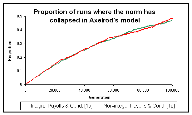
Figure 5. Proportion of runs (out of 1000 for each line) where the norm collapses in Axelrod's model of metanorms. The green line shows runs in which all the payoffs are integers (T = 3; H = –1; E = –2; P = –9; ME = –2; MP = –9) and condition [1b] was implemented. The red line shows runs where every payoff has been divided by ten (T = 0.3; H = –0.1; E = –0.2; P = –0.9; ME = –0.2; MP = –0.9), and condition [1a] was used. The two programs and all the parameters used in this experiment are available in the Supporting Material

Stochastic knife-edge thresholds [3]

8.33

Another interesting example, where the techniques presented in section 8.3 are not always useful, is knife-edge threshold [3] in stochastic models. In contrast to non-stochastic knife-edge thresholds, the important question here is the magnitude of the error in the value of probability, rather than its mere appearance. If such an error is small, then floating-point errors at this threshold will not significantly affect the overall statistical behaviour of the model. This is so because, since the threshold is stochastic, there is no 'wrong branch' in the sense that each one of them would be followed with very similar probability using either arithmetic (given that the error is small by assumption). If the threshold is repeated very frequently in a run, then it would be necessary to ensure that the error is either very small (e.g. if probability is a non-representable constant), or small and unbiased.

8.34

As an example, we study the following knife-edge threshold, which is executed by each agent in BM:

IF(rand < pt) THEN [cooperate] ELSE [defect];

where rand is a random number in the range [0,1] and p_t is the agent's probability to cooperate in time-step t. The probability p_t is updated every time-step according to one of two possible formulae. Which formula is used depends on the action (cooperate or defect) undertaken by each of the two agents in the model in the previous time-step. Because of the simple arithmetic form of the two updating formulae (see Macy & Flache 2002), the error in p_t+1 will be small given any one particular formula. Thus, assuming the same path has been followed in the floating-point model and in its exact counterpart up to a point, the chances of both implementations keep following the same path will be very high. In the unlikely case that the floating-point model deviates from the 'correct' path at some point, one could always argue that such a deviation could have occurred with extremely similar probability in the correct model anyway. Thus, we would conclude that floating-point errors do not significantly affect the overall statistical behaviour of this model.

8.35

To be sure, we re-implemented the BM model in both double precision floating-point arithmetic and exact (rational) arithmetic. We conducted an experiment of 1000 runs, each of them consisting of 2000 iterations, and it turned out that the 2·10⁶ decisions made by each of the agents in the whole experiment were exactly the same in both implementations. Figure 6 shows, for each iteration t, the maximum difference between the values of p_t in each implementation across the 1000 runs. (For the parameterisation used, the value of p_t is the same for both agents in a given implementation). Figure 6 shows that the error is very small, as we had conjectured, but has a clear bias at the end of the runs.

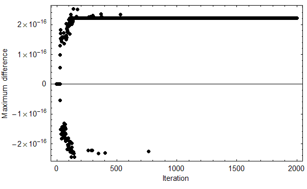
Figure 6. Maximum difference across 1000 runs between the value of pt in an exact implementation of the BM model (Macy & Flache 2002) and the value of pt in an implementation using IEEE 754 double precision arithmetic. The figure shows data for the Prisoner's Dilemma with parameters [π = (4,3,1,0), A = 2, l = 0.5, h = 0, pC,1 = 0.5] (see Macy & Flache 2002). The program used to conduct this experiment is available in the Supporting Material.

8.36

To explain such a bias in the error, it is worth noting that the BM model implicitly relies on infinite precision. It can be analytically proved (Izquierdo et al. 2006) that p_t asymptotically approaches its limit value 1 in every run shown in Figure 6. This asymptotic convergence to 1 is something that could have never been found out for certain using floating-point arithmetic, since there is an infinite set of numbers S (defined as the rational numbers strictly between the largest representable floating-point number smaller than 1 and the number 1) which p_t cannot take in the floating-point implementation but it does take in the exact implementation.

8.37

In fact, the mathematical analysis shows that after a sufficiently high number of iterations in real arithmetic, it is almost certain that p_t takes values in S. However, p_t cannot take any value in the set S in the floating-point model: it either stops at the largest representable number smaller than 1 (or at an even smaller number), or rounds up to 1. In fact, the final value of p_t in every run we conducted with floating-point arithmetic (Figure 6) was 1–2^–52. This value is preserved indefinitely due to floating-point errors. That explains the bias of approximate magnitude 2^–52 ≈ 2.22045·10^–16 shown in Figure 6. In any case, the floating-point model, whilst inexact, is statistically extremely similar to its exact counterpart.

8.38

Thus, we conclude that the overall statistical behaviour of the BM model is not significantly affected by floating-point errors. Admittedly, however, its precise long-term behaviour cannot be adequately studied using floating-point simulations only. Using the parameters shown in the caption of Figure 6, floating-point simulations lock in to an absorbing state^[15], whereas it can be proved that under exact arithmetic no state can ever be revisited! Then again, the exact model does have a limiting state (p_t = 1) that lies near the absorbing state of the floating-point model (p_t = 1–2^–52), and this explains why the macroscopic behaviour of both models turned out to be identical in the 1000 runs we conducted. Thus, it is clear once again that floating-point errors affect certain types of conclusions, but not others – i.e. the importance of floating-point errors in a model strongly depends on the specific use the researcher makes of it.

Summary

9.1

Floating-point arithmetic creates the illusion of working with real numbers, and it does it so effectively that many computer modellers are unaware of the potentially unpleasant effects that it can have on their results. If a model uses floating-point numbers, chances are that it is suffering rounding errors. If, in addition, the model contains knife-edge thresholds, then small floating-point errors may have a disproportionate impact on its results.

9.2

To perform an analysis of the relevance of floating-point errors in a model, the purpose of the model is paramount, since it is the purpose of the model that determines the acceptable magnitude and impact of the errors. In this paper, we have provided a framework intended to assist the reader in finding out whether a particular use of a particular model may be affected by floating-point errors, and what to do about it.

9.3

After conducting an early identification of potential floating-point issues, our next recommendation is to undertake some preliminary tasks aimed at reducing the magnitude of floating-point errors, e.g. appropriate selection of parameter values and re-implementation of mathematical formulae. Small errors affect model results through knife-edge thresholds. Thus, the next step is to conduct a thorough analysis of potentially every knife-edge threshold in the model – interval arithmetic can be very useful at this stage to identify (and dismiss) those knife-edge thresholds where it is certain that the correct branch has been followed, and which therefore do not require further attention.

9.4

The analysis of each knife-edge threshold begins with a characterisation of the set of values involved in its condition part. This characterisation determines which techniques are most useful to ensure that the correct branch of the code is always selected. In this paper, four techniques (tolerance windows, rounding to n significant digits, interval arithmetic, and rational arithmetic) have been described, and their specific strengths and weaknesses have been highlighted.

9.5

Unfortunately, sometimes it is impossible to guarantee that the correct branch will be followed in every knife-edge threshold of a model. In those cases, it is necessary to assess the extent to which following the wrong path affects the conclusions obtained with the model. To do that, we have shown that backward-error analyses are particularly useful: often the magnitude of the impact of floating-point errors can be meaningfully formulated in terms of changes in parameters or slight alterations in the structure of the model. This correspondence between floating-point errors and model structure facilitates the task of determining the relevance of floating-point errors in a certain model that is being used for a certain purpose.

Acknowledgements

This work has been funded by the Scottish Executive Environment and Rural Affairs Department. We would like to thank Bruce Edmonds for many helpful comments and discussions, Dale Rothman for suggesting the term 'knife-edge', Nick Higham for useful advice at the early stages of this investigation, and three anonymous referees for their clarifying suggestions.

Notes

¹The most common base in floating-point computing systems is base 2.

²Some authors refer to control flow statements, rather than branching statements. By branching statement we mean any point in the code of a program where the flow of control may diverge. Some examples are:
IF(condition)THEN(action), and
DO(action)WHILE(condition).

³It is also assumed that nu < 1.

⁴RAEAN stands for "Reimplementation of Axelrod's 'Evolutionary Approach to Norms' " (Galán & Izquierdo 2005).

⁵In the BM model it is necessary to multiply the aspiration level by the same constant too.

⁶By 'digits of a real number x' in a certain base b we mean the minimum number of digits X necessary to write x in base b, according to the format X·X…X · b^exp, and without loss of precision.

⁷Even if {x_i} were large, one could always subtract an integral estimate of the mean of {x_i} from every x_i, and then apply [1b] to the shifted data.

⁸Please note that at this stage we are only concerned about the first appearance of floating-point errors, not about the impact of such errors in evaluating the condition. Even if the condition is evaluated correctly in both implementations, implementation [1b] will help us to focus on the relevant errors in the model (e.g when doing an automatic detection of all the errors). The same applies for [2a] and [2b].

⁹We arrived at this statement using interval arithmetic. Later in the paper we acknowledge interval arithmetic as a useful technique to identify those knife-edge thresholds where the correct branch of the code has been followed for certain, and which therefore do not require any further attention.

¹⁰Knuth (1998, p. 233) also suggests a variation on this approach that takes into consideration the magnitude of the operands. A brief investigation using CharityWorld did not find this improved things much (Polhill et al 2006).

¹¹It is also assumed that both numbers lie within the range of normalised floating-point numbers. In double precision that range is: [–1.797…·10³⁰⁸, –2.225…^–308] ∪ [2.225…^–308, 1.797…·10³⁰⁸].

¹²If errors are not too large, this means that when the wrong branch is followed, it is because two numbers that should have been equal are detected as different (due to small floating-point errors), which is most often the case.

¹³In our experiments it turned out that using integral parameters was enough to select the right branch at the knife-edge threshold every time the condition was evaluated: the 1000 runs we conducted with implementation [1b] and integral payoffs produced exactly the same results as the 1000 runs we conducted with implementation [1a] and integral payoffs.

¹⁴Interestingly, these tests also showed that the error is somewhat biased.

¹⁵The value of p_t completely determines the state of the system.

Appendix A

The following two theorems provide the theoretical basis to show that using tolerance windows of magnitude ε = [d_min/3] _f– , the correct path in a branching statement is always followed as long as the absolute error in each number to be compared is less than ε/2.

Theorem 1: Let x, y and ε (ε ≥ 0) be three floating-point numbers and assume that summation and subtraction are exactly rounded (as the IEEE 754 standard stipulates). If |x – y| > 2ε, then x and y will be detected as being different using tolerance windows of magnitude ε.

Proof: Assume for now that x > y. Then |x – y| > 2ε implies that x > y + 2ε. Let D(y + ε) be the error in computing [y + ε]_f, expressed as D(y + ε) = [y + ε]_f – (y + ε). It can be easily shown that |D(y + ε)| ≤ ε. Thus,

x > y + 2ε ⇒ x > y + ε + D(y + ε) ⇒ x > [y + ε]_f

The proof for the case where x < y is analogous. The 2ε margin is the smallest needed to guarantee that the two numbers will be detected as different, since there are cases where |x – y| = 2ε and the result of this proposition does not apply. ¤

Theorem 2: Let x, y and ε be three floating-point numbers and assume that summation and subtraction are exactly rounded (as the IEEE 754 standard stipulates). If |x – y| ≤ ε then x and y will be detected as being equal using tolerance windows of magnitude ε.

Proof: |x – y| ≤ ε ⇔ y – ε ≤ x ≤ y + ε

Since subtraction is exactly rounded, we know that [y – ε]_f ≤ x. This is because x is a floating point number that is nearer to y – ε than any floating point number greater than x (since y – ε ≤ x ). Similarly, we also know that x ≤ [y + ε]_f. Assuming a larger margin for |x – y| would not provide such a guarantee. Thus, if |x – y| ≤ ε, then [y – ε]_f ≤ x ≤ [y + ε]_f . ¤

In summary, if summation and subtraction are exactly rounded, then using tolerance windows of magnitude ε will enable the model to follow the correct branch if:

1. Each pair of numbers that need to be detected as different for the model to follow the right branch are correctly ordered, and their absolute difference is greater than 2[ε]_f.
2. No two numbers that need to be detected as being equal for the model to follow the right branch have an absolute difference greater than [ε]_f.

It can be easily proved that setting ε = [d_min/3] _f– guarantees both (i) and (ii) above as long the absolute error in each number is less than ε/2.

Appendix B

Appendix B is here.

Appendix C

Appendix C is here.

References

AXELROD R M (1986) An Evolutionary Approach to Norms. American Political Science Review, 80 (4). pp. 1095-1111.

BOOCH G, Rumbaugh J, and Jacobson I (1999) The Unified Modeling Language User Guide. Addison-Wesley, Boston, MA.

CHAN T F, Golub G H, and LeVeque R J (1983) Algorithms for Computing the Sample Variance: Analysis and Recommendations. The American Statistician, 37(3). pp. 242-247.

FLACHE A and Macy M W (2002) Stochastic Collusion and the Power Law of Learning. Journal of Conflict Resolution, 46 (5). pp. 629-653.

GALÁN J M and Izquierdo L R (2005) Appearances Can Be Deceiving: Lessons Learned Reimplementing Axelrod's 'Evolutionary Approach to Norms'. Journal of Artificial Societies and Social Simulation, 8 (3), https://www.jasss.org/8/3/2.html

GOLDBERG D (1991) What every computer scientist should know about floating point arithmetic. ACM Computing Surveys 23 (1). pp. 5-48.

GOTTS N M, Polhill J G, and Law A N R (2003) Aspiration levels in a land use simulation. Cybernetics & Systems 34 (8). pp. 663-683.

HIGHAM N J (2002) Accuracy and Stability of Numerical Algorithms, (second ed.), Philadelphia, USA: SIAM.

IEEE (1985) IEEE Standard for Binary Floating-Point Arithmetic, IEEE 754-1985, New York, NY: Institute of Electrical and Electronics Engineers.

IZQUIERDO L R, Gotts N M, and Polhill J G (2004) Case-Based Reasoning, Social Dilemmas, and a New Equilibrium Concept. Journal of Artificial Societies and Social Simulation, 7 (3), https://www.jasss.org/7/3/1.html

IZQUIERDO L R, Izquierdo S S, Gotts N M, and Polhill J G (2006) Transient and Long-Run Dynamics of Reinforcement Learning in Games. Submitted to Games and Economic Behavior.

JOHNSON P E (2002) Agent-Based Modeling: What I Learned from the Artificial Stock Market. Social Science Computer Review, 20. pp. 174-186.

KAHAN W (1998) "The improbability of probabilistic error analyses for numerical computations". Originally presented at the UCB Statistics Colloquium, 28 February 1996. Revised and updated version (version dated 10 June 1998, 12:36 referred to here) is available for download from http://www.cs.berkeley.edu/~wkahan/improber.pdf

KNUTH D E (1998) The Art of Computer Programming Volume 2: Seminumerical Algorithms. Third Edition. Boston, MA: Addison-Wesley.

LEBARON B, Arthur W B, and Palmer R (1999) Time series properties of an artificial stock market. Journal of Economic Dynamics & Control, 23. pp. 1487-1516.

MACY M W and Flache A (2002) Learning Dynamics in Social Dilemmas. Proceedings of the National Academy of Sciences USA, 99, Suppl. 3, pp. 7229-7236.

POLHILL J G, Gotts N M, and Law A N R (2001) Imitative and nonimitative strategies in a land use simulation. Cybernetics & Systems, 32 (1-2). pp. 285-307.

POLHILL J G and Izquierdo L R (2005) Lessons learned from converting the artificial stock market to interval arithmetic. Journal of Artificial Societies and Social Simulation, 8 (2), https://www.jasss.org/8/2/2.html

POLHILL J G, Izquierdo L R, and Gotts N M (2005) The ghost in the model (and other effects of floating point arithmetic). Journal of Artificial Societies and Social Simulation, 8 (1), https://www.jasss.org/8/1/5.html

POLHILL J G, Izquierdo L R, and Gotts N M (2006) What every agent based modeller should know about floating point arithmetic. Environmental Modelling and Software, 21 (3), March 2006. pp. 283-309.

WILENSKY U (1999) NetLogo. http://ccl.northwestern.edu/netlogo/. Center for Connected Learning and Computer-Based Modeling, Northwestern University, Evanston, IL.

SUN MICROSYSTEMS (2000) Numerical Computation Guide. Lincoln, NE: iUniverse Inc. Available from http://docs.sun.com/source/806-3568/.

Return to Contents of this issue

© Copyright Journal of Artificial Societies and Social Simulation, [2006]