
Introduction
A common feature of financial markets since their advent has been periods where price movements and trading volumes have been much larger than what is commonly experienced; that is, the markets become more volatile. The semi-regular appearance of bubbles, defined as an “upward price movement over an extended range that then implodes”, (Kindleberger & Aliber 2011) has left academia and the general public searching for answers. Debate continues on whether it is even possible to predict future movements of the financial markets and whether a bubble can even be detected in advance (e.g. Gupta, Hauser & Johnson, 2005). The “mainstream” doctrine and practices in financial markets have tended to follow Fama’s (Fama 1970) Efficient Market Hypothesis (EMH), which states that an asset’s price fully reflects all available information. Despite some empirical support for the EMH, the reality of continued episodes of boom and contradictory pioneering statistical evidence from the likes of Bollerslev, Engle and Nelsonc(1994) and Mandelbrot (1963), provides evidence that markets may not function in accordance with the EMH.
An alternate approach to the EMH is to consider financial markets as a complex adaptive system (CAS). To consider a financial market as a CAS is to accept that its behavior results from an emergent process, which occurs via the self-organized behavior of independently acting, self-motivated individuals (Farmer et al. 2012). Sornette (2014) succinctly defined the relevance of the CAS approach to financial markets when he concluded after 20 years of research that the key concepts required to understand stock market returns are, imitation, herding, self-organized co-operativity, and positive feedbacks, which are all properties of a complex system.
The CAS framework has the further advantage of allowing researchers to consider the impacts networks within their analytical framework. The justification for utilizing networks is that the behavior of a system has been found to vary greatly depending on the network structure (the topology) of the system. Classic papers that demonstrate the implications of different network topologies include: Albert, Jeong, & Barabási (2000), Santos and Pacheco (2005), and Callaway et al. (2000). The existence of networks between investors and their relevance to financial markets was raised by Shiller and Pound (1989), whose research found evidence that personal contact had an impact on the decisions of investors. Further support is provided by Hong, Kubik, & Stein (2005) who found evidence that professional fund managers spread information, via word of mouth, that resulted in investment decisions.
Given the characteristics of a CAS, traditional analytical approaches are rendered ineffective, and researchers have been forced to turn to computer simulation to understand their dynamics. ABMs have become one of the key tools in trying to understand the dynamics of a CAS. Squazzoni (2010) provides a comprehensive review of the important contributions that ABMs have made in progressing the social sciences, including how, amongst other things, it has promoted a generative and trans-disciplinary approach to solving problems. The utility of ABMs to the field of economics is detailed by Hamill and Gilbert (2016), where they demonstrate how ABMs not only complement the traditional modelling approaches but how through bottom-up modeling they are able to combine the micro and macro aspects of a system.
The remainder of this paper is structured in the following manner: the background to and the support for this paper, followed by a review of the model underlying this paper, including both the original model of Harras and Sornette (2011) and the authors’ extension, which include the use of differing network topologies and the introduction of multiple risky assets. The results selection follows and is split into two sub-sections: the single risky asset model utilizing varying topologies followed by outcomes of the multi-asset model. A conclusion and discussion are provided to summarize the significance of the findings and highlight future research opportunities.
Background
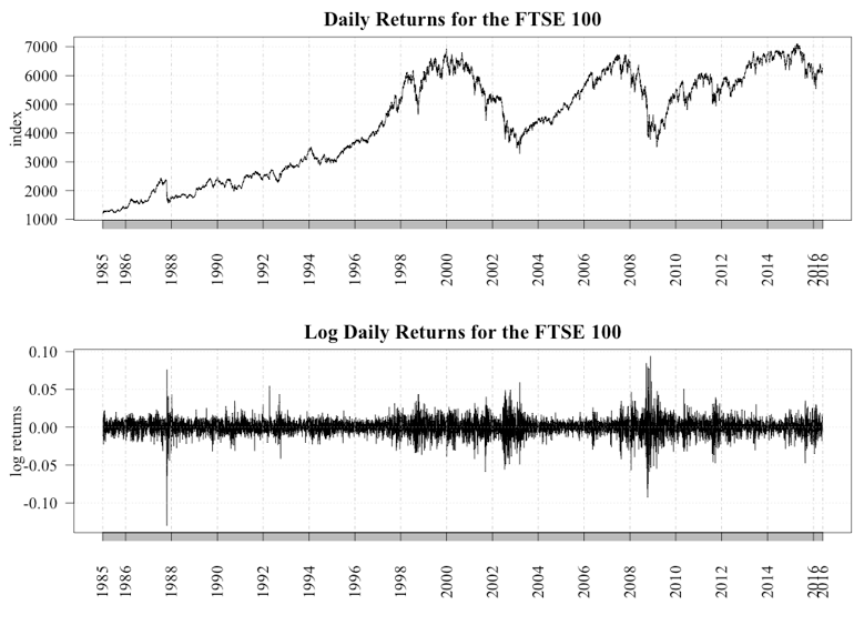
A key assumption of the EMH is that the price of an asset reflects all current and known information, and, because news arrives in a random unpredictable fashion, prices will follow a similar pattern, which is one of a random walk. This implies that returns should follow a Gaussian distribution and asset bubbles and subsequent crashes will not and cannot occur. However, a review of Figure 1, which charts the movement of the FTSE 100 index and its daily log returns between 1985 and 2016, shows that while at times the returns have followed the random walk as prescribed by the EMH, there have been several incidences where returns have deviated greatly, such as 1987 and 2007. The significance of these large deviations was seen when the global markets crashed in 2007 and the world plunged into the Global Financial Crisis (GFC), which according to the IMF cost the global economy $USD11.9 trillion (Conway 2009). Given the potential cost associated with the periods of extreme volatility, to this author a theory consistent with “close enough is good enough” does not suffice.
An alternative interpretation of the return characteristics of financial markets, as summarized by Cont (2007) and Johnson, Jefferies, & Hui (2003), is that they demonstrate a set of stylized facts that include: excess volatility – the existence of large movements not supported by the arrival of new information; heavy tails – returns exhibit “heavy tails” or “fat tails,” indicating returns deviate more than anticipated and do not follow a Gaussian distribution; volatility clustering – large changes are followed by further large changes; and volume/volatility clustering – trading volumes and volatility show the same type of long memory. In addition to these stylized facts, Mandelbrot (1963) provided evidence that returns followed a very unique distribution, a power law distribution. Lux (2016) provides a detailed review of the empirical evidence supporting the existence of power laws in financial markets. For investors, the main implication of returns following a power law is that the risk of large losses is much higher than suggested by the EMH. The existence of power law returns suggests the presence of a complex system, thus providing insight into a mechanism that can generate such returns.
To gain an understanding of the dynamics of a complex system, ABMs have become a key tool as they allow for interaction between individual agents – investors, in the case of financial markets - who act and undertake actions based on the context of their environment utilizing basic rules. The agents’ behavior is not fixed and can evolve in response to the behavior of other agents and their environment. Therefore, ABMs are not constrained to equilibrium conditions (Sornette 2014), which is a key assumption underlying traditional neo-classical models of finance and economics in general.
While there is a large volume of work utilizing ABMs to simulate financial market returns (see LeBaron 2006 and Sornette 2014) for extensive reviews of the application of ABMs to financial markets), there has been a limited utilization of networks within the various models. This is most likely because the research effort, which commenced before the explosion of network theory in the 2000’s, was so computationally intensive that there was little capacity remaining to overlay a network topology at the time. The benefits of adding networks has since been demonstrated by Hoffman, Jager and Von Eije (2007), who matched real-world market returns in a model that utilized social interaction amongst investors; Panchenko, Gerasymchuk and Pavlov (2013), who showed that network structures were capable of influencing the stability of, and the fluctuations of, an asset’s price; and Harras and Sornette (2011), who demonstrated how bubbles may emerge as a result of agents considering different information sources, including the expected actions of their neighbors.
A shortcoming of the literature relating to ABMs and artificial stock markets is their utilization of a single risky asset and a risk-free asset, therefore reducing the problem to one of asset allocation rather than choosing amongst many risky assets. In the real-world, investors are not only faced with the decision of how to allocate their wealth across asset classes but also within those asset classes. For example, a typical investor will invest in domestic and international bonds, domestic, international and emerging market equities, and various alternative assets. This process is undertaken in an attempt to diversify the risk of their investments.
Complicating the process is the degree by which assets are correlated, and how that correlation changes, especially in times of financial distress when the asset correlation increases in general.
This paper implements an ABM designed to test the impact that the different network structures have on the performance of financial markets, and whether certain network structures generate greater volatility. The model can identify the dynamics that influence whether, or not investors form large common groups (“herds”) in terms of their investment strategies. Understanding the dynamics of herd formation is important as it provides insights into how and why bubbles form and collapse in financial markets. The model is also capable of investigating the causation of several documented impacts of investor networks, including, how the topology of a social of network impacts information efficiency (Ozsoylev and Walden 2011) and the role that centrality plays in determining the dynamics of the market (Ozsoylev et al. 2014; Walden 2014).
Additionally, in what is believed to be a first for an artificial stock market, this paper introduces the ability for agents to consider multiple risky assets. The rationale for this inclusion is to see if, and under what circumstances, if any, agents with basic rules can successfully diversify their portfolio in line with traditional financial theory. Another advantage of introducing multiple assets into a model is to allow, in future iterations of the model, firms to become heterogeneous agents in their own right, thus allowing them to react to their environment, with decisions such as divided policy and capital investment potentially becoming endogenous. The utility of such an approach has been demonstrated by Grebel and Merey (2009).
Methodology
To achieve the goals of the research, the ABM developed by Harras and Sornette (2011) formed the foundation of the implemented model, the justification being that the original model produced price movements that were affected by how strongly agents were influenced by their neighbors. This resulted in asset returns that were fat-tailed, which was inconsistent with the Gaussian distribution of the public and private information used by the agents. Another key discovery was the presence of a phase transition when the coefficient with regards to the initial bias investors had towards the information coming from the network was increased beyond a critical level. The explanation for the change in behavior beyond the critical point was that a positive feedback loop relating to investors adapting the actions of their neighbors became material and investors began to “herd.”
Figure 2 provides an illustration of the steps taken in the model. A brief description of the original model and the authors’ extensions follows, while a detailed overview, design and details (ODD) document, and source code are available at https://www.openabm.org/model/5203/). The author’s model was implemented in NetLogo 5.3 (Wilensky 1999) with the agents initialized as per the NetLogo default of a random asynchronous order with the time period per step being a quarter. A further discussion of the initial conditions and the analytical methodology used in this paper is contained in the Verification section.
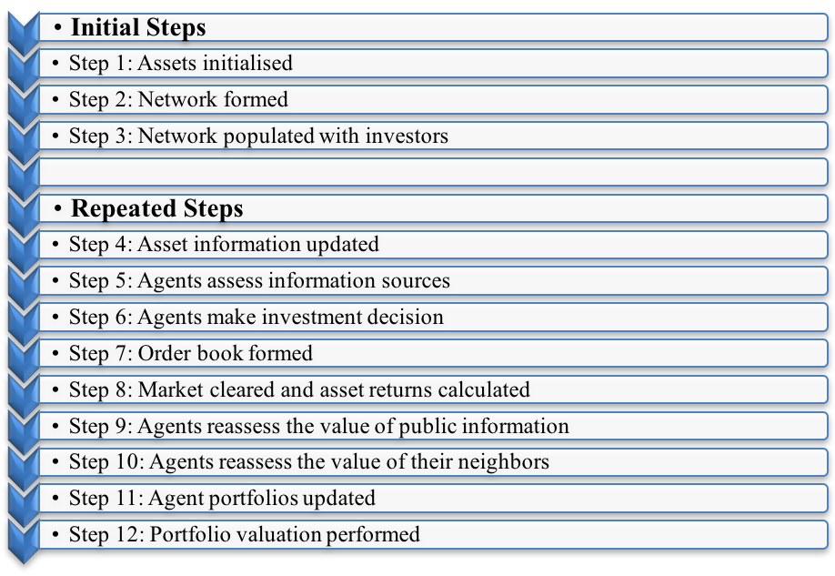
The purpose of the model is to have boundedly rational investors allocate their wealth between the risk-free asset (a proxy for cash) and a risky asset. The investors utilize Equation 1 to decide whether they wish to buy, hold or sell more of the risky asset at each time step. The agents’ holdings of the risk-free asset will either decrease as it is used to buy more of the risky asset or increase from the proceeds of selling some of the risky asset. Once investors make their investment decision they transact via the artificial stock market, with a new price for the risky asset(s) endogenously determined based on the relative demand and supply for the risky asset. This process allows a variety of accompanying asset price and portfolio statistics to be calculated. Finally, investors reassess the level of trust (\(nt_{jk}\wedge pt_i\)) they have in the information coming from the public source (pii(t)) and their network (Eij[aik(t)]), dependent on whether it provided the correct advice. That is, if the information tells the agent to invest and the price subsequently increases, then the agent will increase the trust in that source. Alternatively, the trust will decline if the price falls following a buy signal from the information source
| $$\omega_{ij}=c_{1\,ij}\Biggl(\sum_{k=1}^Knt_{jk}(t-1)E_{ij}[a_{ik}(t)] \Biggr)+c_{2\,ij}\, pt_i(t-1)\,pi_i(t)+c_{3ij}\,\epsilon_{ij}(t) $$ | (1) |
The relevant definitions for Equation 1 are: ωij is the decision score for the jth agent with relation to the ith asset (I being the total number of assets); (Eij[aik(t)]) is the estimated action of agent j’s kth neighbor in relation to asset i at time period t; pii(t) is the public information, which is the same for all agents, for the ith asset at time period t and εij(t) is defined as the private information of the jth agent for the ith asset for the time period. K refers to the number of neighbors agent j has, where agent j’s neighbors are those agents it is connected to via the given network structure.
Equation 1 is implemented such that the level of influence of each information source is weighted by two variables (the exception is private information, which has a single fixed variable), with one fixed and the other updated at each time-step. The fixed values are given by c1ij, c2ij and c3ij, where the c variable relates to the information source (neighbors (c1), public (c2) and private (c3)) and i and j relating to the value for the jth agent for the ith asset. The agent’s values for c1ij, c2ij and c3ij are set by the user and it is by altering the c1ij, c2ij and c3ij coefficients that different dynamics are generated, including the appearance of bubbles in the risky asset’s price. The variable coefficients are network trust (ntjk) and public trust (pti), with ntjk being the trust agent j has in neighbor k, and pti being the trust in public information for asset i. Given the nature of public information, all agents maintain the same level of trust in the source.
The multi-asset extension
The inclusion of multiple risky assets overcomes a key shortcoming of previous artificial stock markets. The extended model allows for up to ten assets (as defined by I) thus allowing portfolio analysis to be considered, which in turn allows the production of a dynamic efficient frontier, the benefit of which is beyond the scope of this paper.
The introduction of multiple-asset model required various modification in terms of how the updating of the two trust variables occurred. It was decided that for public trust the population would maintain trust at an individual asset level to preserve the heterogeneous nature of the asset’s performance as defined in Equation 2. In contrast, in determining the trust for each of their neighbors, an investor will assess that neighbor’s individual recommendations before updating the trust based on the average performance of those recommendations as shown in Equation 3. The significance of this difference is that for an agent to generate a high level of trust in a neighbor, that neighbor must consistently provide the correct action for all assets, and is not trusted for being an expert in any one asset. Opposed to this, an investor may grow to trust the public information of one asset more than another, which is akin to the assets having varying levels of “efficiency” as dictated by the EMH.
| $$pt_i(t)=\alpha pt_i(t-1)+(1-\alpha)\,pi_i \frac{(t-1)*r_i(t)}{\sigma_{ir}(t)} $$ | (2) |
| $$nt_{jk}(t)=\frac{\sum_{i=1}^I\alpha\,nt_{jk}(t)+(1-\alpha)E_{ij}\frac{[a_{ik}(t)]*r_i(t)}{\sigma_{ir}(t)}}{I} $$ | (3) |
For the single-asset model, public information is determined by a Gaussian white noise process with a mean of 0 and variance of 1 (N(0,1)). To allow for the varying effects of multiple assets, two changes were made. The first dealt with the question of how correlated the assets are to each other. To allow for this, the public information of the assets can be adjusted to be fully, partially, or not at all correlated. This is achieved by the public information of the assets being correlated to the first asset (Asset 0) by the corr_r parameter (the β value in Equation 4), with the value set as a constant for all risky assets in the range of 0 to 1. In addition, the standard deviation of each asset is increased by 10% to maintain a level of heterogeneity.
| $$pi_i(t)=\beta * AssetNews_0(t)+(1-\beta) AssetNews_i(t) $$ | (4) |
The public information for each asset at each time period is given by Equation 4. The process by which it is generated is that the news for the first asset (asset 0) is first randomly chosen from the Gaussian distribution, with the process repeated for each of the assets. The final value for each asset, other than asset 0, is then determined by weighting the values by β or 1 - β. The equation only addresses the pair-wise correlation between the first asset and each subsequent asset, but if β = 1 then all risky assets will have the same public information.
The network extensions
Within network science literature there are four general types of network: regular/lattice; random (Erdos-Renyi model); small-world; and scale-free. In high-level terms, the differences relate to how each agent is assigned its neighbors and the number of neighbors it has. These small differences can generate non-trivial differences in the outcome of the system and for the agents within the network.
In terms of generating the networks, except for the Erdos-Renyi network, where the network extension of NetLogo was utilized, user-designed algorithms were used that, depending on the network, made use of the following variables:
ring_M– Controlled the number of neighbors in a lattice network or the number of hubs in the scale-free network (Barabási & Albert 1999);prob_of_rewire– Controlled the probability of an agent rewiring in a small-world network as detailed by Watts and Strogatz (1998); andprob_of_link– Controlled the probability of an agent connecting either to a hub or another agent following the theory of a random graph as per Erdös & Rényi (1960).
The implemented approach ensured that the number of edges (5,000) and the average number of neighbors (4) would be consistent across the different network structures. Therefore, any difference in the outcome was not influenced by the number of edges, but solely by the degree distribution of the networks. Therefore, if an investor has only one neighbor it will have an initial bias towards public and private information, as it collects less opinions, and if it has a lot of neighbors there will be an initial bias to the information coming from the network as they collect more opinions. Consideration was given to normalizing the network score but this would minimize the impact of the different network structures. In addition, as investors continually reassess their trust in each information source, it does not preclude a single neighbor becoming very persuasive. Conversely, an investor with many neighbors may end up developing very little trust in those neighbors.
Model output
Given the nature of the model the most important output is the price of the risky asset(s) as determined by the market clearing process at each step, which allows the asset’(s’) returns to be calculated. It is the statistical characteristics of these variables that form the focus of analysis within this paper. In addition, the level of aggregate network trust is analyzed to assess the role it plays in price dynamics.
Verification
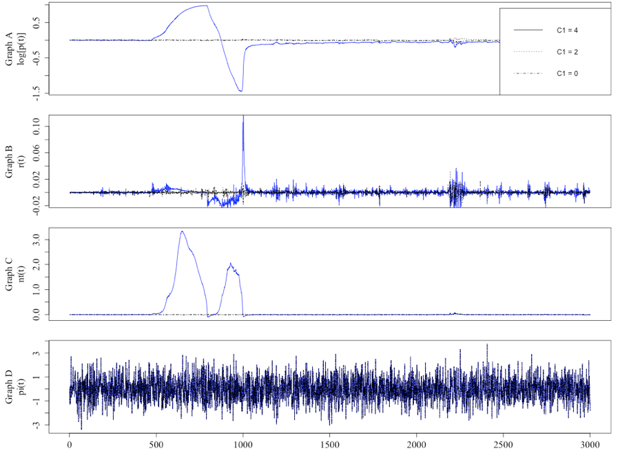
The first step of the verification process was to ensure the extended model matched the output of Harras and Sornette (2011). Figures 2 and 3 are representative runs of the author’s model, selected such that the results illustrated a close match in terms of the level and variation of the key variables when compared to the equivalent Figure 1 and 2 in Harras and Sornette (2011). Figure 2 shows that the price and returns under the default settings (as displayed in Table 1) are not non-normally distributed, when compared to the public information, and that the price becomes more volatile as the level of trust in the network information increases. Figure 3 illustrates the impact on the risky asset’s price by varying c1ij. It highlights the presence of an excitable regime when c1ij is set at 4.
| Variable | Setting |
| Steps per run/ Number of runs per setting | 3,000/50 |
| Number of investors | 2500 |
| Conviction threshold | 2 |
| Market depth (λ) | 0.25 |
| Transaction ratio | 0.02 |
| Memory length (α) | 0.95 |
| Initial bias to all information | 1 |
In terms of an analytical framework used in the following section, in contrast to Harras and Sornette (2011), who made use of the maximum draw-up and draw-down, this paper utilizes the mean and the standard deviation of the price series to highlight how the initial conditions affected the behavior of the system. The use of a “burn in” period is not utilized in either paper, with 3,000 steps per run chosen as the analytical base for this paper. The rationale being that it allows sufficient time for the system to normalize after a bubble should it occur. The main justification for not utilizing a “burn in” period is that the price of the asset is initialized at its justifiable equilibrium prices, that is a price of 1, and with the public and private news being normally distributed with a mean of 0 and a standard deviation of 1, outside the influence of the network topology, and the bias investors have towards listening to their neighbors, the asset’s price should move as per a simple random walk, with it the mean price remaining around 1. In more general terms, the price starts at what is the model’s ultimate attractor, thus eliminating the requirement for an initial transient period to allow the model to move towards a steady state attractor.
It should be noted that with the model having the ability, albeit unpredictably, to form a positive feedback with regards to the neighbors influencing each other, there should be no expectation that the system should reach a steady state close to the justifiable equilibrium of 1. Justification firstly comes from Harras and Sornette (2011), who highlight that the only reason a bubble collapses in their model is that investors run out of funds to invest, and if they had access to further funds the asset bubble would continue to grow. In turn, the market fails to reflate the bubble because while bullish investors remain and still form buying herds, they have insufficient funds given the loss of their capital due to the market collapse. Alternatively, the market can demonstrate excess volatility indefinitely if investors are not drawn into a market bubble that drains them of all their resources. Ultimately, the system will display different behavior pre-and and post-bubble, and while a detailed analysis is outside the scope of this paper, an appendix is provided which provides an example of this differentiated behavior.
In terms of how many runs per setting were made 50 was chosen as it was a satisfactory compromise between generating sufficient samples, to ensure the validity of the statistical tests, and resources required to generate those results, as the collection of the model’s output at each time-step became computationally expensive.
More precise back to back testing to verify the author’s model was not able to be undertaken due to an inability to access the code for the original model. This point, as raised by Janssen (2017), is an ongoing issue in the agent-based modeling community, whether the sharing of code is not common practice.
Other verification steps included: the generation of a journal to allow for manual calculations to be undertaken to ensure calculations within the model were correct; visual inspection of various charts plotting the behavior of the variables; a code walk-through to produce flow charts to ensure the code implemented the intended model; and parameter sweeps of the extreme values.
Results and Findings
The parameter sweeps for the various scenarios were performed with the characteristics as per Table 1, except for the bias toward network information, which was varied between 1 and 4. This is in line with the focus of the paper, which is to analyze the volatility of the market resulting from varying the network structures and the level of initial bias investors have in their network information (the c1 variable). The network structures utilized in the model and their exact characteristics for the experiments are detailed in Table 2.
| Network | Key Characteristics |
| Lattice | Number of links per investor = four |
| Small-world | Number of initial links per investor = four The probability of rewiring = .10 |
| Erdos-Renyi | Probability of connection = .0016 |
| Scale-free | Number of hubs = 10 Probability of connection = .20 |
Table 3 provides a summary of the various metrics that may provide insights into the varying behavior across the topologies of the networks used. The results show that while the average number of neighbors for each of the networks is 4 (refer to (a) in Table 3), the distribution is varied (refer to (b) in Table 3), with the lattice having a uniform degree distribution, while the scale-free network has the largest standard deviation, suggesting a highly skewed distribution in line with the distribution prescribed by a scale-free network. The scale-free network’s clustering coefficient is in the middle of the sample, while the lattice and Erdos-Renyi network are at either end of the spectrum (refer to (c) in Table 3). Therefore, we would expect the scale-free network to be the most volatile and the others to be less volatile if the results of Ozsoylev and Walden (2011) hold.
| Topology | Neighbors | Closeness | Clustering | Betweeenness | |
| Max. | Lattice | 4 | 0.0032 | N/A | 389,688 |
| Small-world | 7 | 0.1272 | N/A | 126,773 | |
| Scale-free | 562 | 0.5268 | N/A | 441,143 | |
| Erdos-Renyi | 13 | 0.2124 | N/A | 38,291 | |
| Average | Lattice | (a) 4 | 0.0032 | (c) 0.500 | 389,688 |
| Small-world | (a) 4 | 0.0976 | 0.380 | 11,646 | |
| Scale-free | (a) 4.0208 | 0.3361 | (c) 0.141 | 1,694 | |
| Erdos-Renyi | (a) 4.0446 | 0.1723 | (c) 0.002 | 5,631 | |
| Std. Dev. | Lattice | (b) N/A | N/A | N/A | N/A |
| Small-world | (b) 0.6204 | 0.0083 | N/A | N/A | |
| Scale-free | (b) 31.774 | 0.1199 | N/A | 24,965 | |
| Erdos-Renyi | (b) 2.01 | 0.0292 | N/A | 5,422 |
The impact of varying network topology
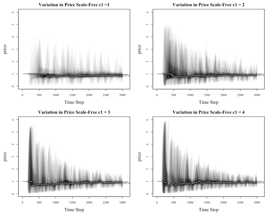
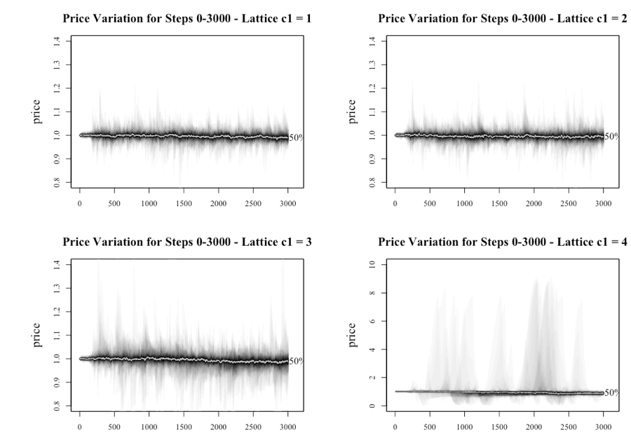
The impact on the price of the asset from varying levels of c1ij (detailed in the heading by the c1 value, for convenience the terms c1 and c2 will be used to describe the upper limit of the c1ij and c2ij terms) across the varying network structures is seen in Figure 5 and 6. For the fan plots (Abel 2015), the reader should note that the x-axis in these charts is time as determined by the step number of the experiment. The plots have the median price for the sample shown with the line marked with 50%. The differences for the various levels of c1 and networks are detailed in Table 4 and 5. The reader should also note that the axes for c1 = 1 to 3 are the same before increasing when c1 is set to 4 under a lattice network.
The results from the lattice network are consistent with the original model as it is not until the level of c1 is greater than 2 that the system starts to deviate in any meaningful manner from a price level of 1. The existence of bubbles and crashes, demonstrated by the price approaching 8 and 0, is seen when c1 is equal to 4. The fan plots for small-world and Erdos-Renyi networks are not dissimilar to the lattice network.
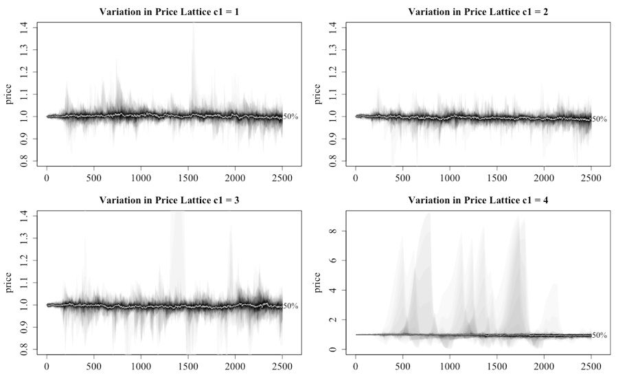
The behavior of the scale-free network, as illustrated in Figure 6, is materially different from the other networks as witnessed by the dramatic price movements, regardless of the setting level for c1. This finding delivers the first key finding of this paper. In another interesting result, the level of c1 does appear to affect the peak of the initial bubble. There also appears to be a trend where the price oscillates, with each oscillation decreasing in magnitude. The reappearance of the bubbles but at lower peaks relates to the gradual loss of wealth for the investors who are caught in the boom and bust cycle. Another point is that once the initial bubble implodes, the median price dips below 1, as the herd stampedes to the exit in the first crash, before gradually increasing throughout the remainder of the run as investors return to market.
A more conclusive view of how the prices (and therefore returns) vary for the various networks is provided by the boxplots in Figure 7 (the mean price per series) and Figure 8 (the standard deviation of each series). The data for the plots comes from finding the mean price and the standard deviation from the 50 runs of 3,000 steps for each of the settings in the parameter sweep.
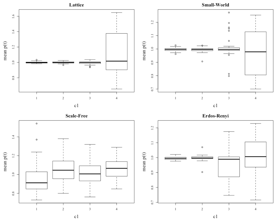
Figure 7 illustrates that as c1 increases, the volatility in all the networks starts to increase. However, the level of volatility is not consistent across the networks, and this is the second finding of significance of this paper. The difference in the volatility of the networks is seen more clearly in Figure 8, which displays boxplots of the standard deviation of the prices within the different scenarios.
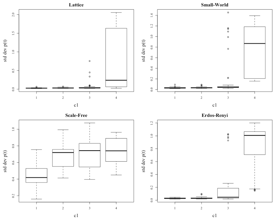
It appears that increasing c1 influences the volatility of the system, regardless of the network topology. This holds for even the scale-free network, which has higher volatility at the initial level of c1 = 1, despite not increasing as much across the spectrum of c1. The volatility of the remaining networks increases once c1 = 3, as seen by the appearance of outliers. Another point of note is that the distributions are heavily skewed for all networks except the scale-free network.
Table 4 provides the mean prices for the various combinations of c1 and the network type, along with the overall average and p-values for testing the null hypotheses, that there is no difference in the mean of the price series. To test for the statistical significance for the various combinations, Kruskal-Wallis rank sums tests were performed as the returns of the mean and standard deviations were not normally distributed.
The first hypothesis test was to see whether, for a given level of c1 there were no differences in the mean of the price for the various network types. The p-values are provided in the p-value column or row. The null is rejected as the mean price of the various networks are statistically different (see (a) in Table 4 ). Varying the level of c1 also statistically alters the mean price when all networks are considered (see (b) in Table 4 ). For the different network types, it is only the scale-free network that has a statistically different mean price after varying the level of c1 (see (d) in Table 4 ).
A second set of tests was used to determine whether there were differences in the mean of the price for the various levels of c1 for each of the networks. The null is rejected when c1 is set at 1 or 2 as the mean prices for the individual networks are statistically different (see (c) in Table 4 ). The lack of difference between the mean prices once c1 is increased to 3 or beyond is significant and, as discussed later, the network topology becomes irrelevant when investors favor listening to their neighbors over fundamental analysis.
| Network Influence c1ij | Average | p-value | ||||
| Network | 1 | 2 | 3 | 4 | ||
| Lattice | 0.999 | 0.999 | 0.995 | 1.108 | 1.025 | 0.161 |
| Small-world | 0.997 | 0.995 | 1.008 | 0.977 | 0.994 | 0.863 |
| Scale free | 0.955 | 1.047 | 1.020 | 1.055 | 1.019 | (d) <0.01 |
| Erdos-Renyi | 0.996 | 0.998 | 0.952 | 1.010 | 0.989 | 0.079 |
| Average | 0.987 | 1.010 | 0.994 | 1.038 | 1.007 | (b) <0.01 |
| p-value | (c) 0.019 | (c) 0.027 | 0.083 | 0.080 | (a) 0.037 | |
Table 5 provides the average standard deviation of the prices for the various combinations of c1 and network type, along with the overall average and statistical significance of any differences. Hypothesis tests similar to those performed previously show that the standard deviations of the prices across the various networks are statistically different (see (a) in Table 5). Also, when c1 is set at 1, 2 or 3 the standard deviation for the various networks is statistically different (see (c) in Table 5). However, once c1 is set at 4 the level of volatility within the system is not statistically different (see (d) in Table 5). Additionally, the standard deviation of the prices within the networks is statistically different (see (b) in Table 5), yet across the different network topologies, it is only the scale-free network that has a statistically different standard deviation with varying levels of c1 (see (e) in Table 5).
| Network Influence c1ij | Average | p-value | ||||
| Network | 1 | 2 | 3 | 4 | ||
| Lattice | 0.028 | 0.033 | 0.068 | 0.746 | 0.219 | 0.161 |
| Small-world | 0.032 | 0.035 | 0.176 | 0.740 | 0.246 | 0.863 |
| Scale free | 0.427 | 0.669 | 0.698 | 0.730 | 0.631 | (e) <0.01 |
| Erdos-Renyi | 0.029 | 0.033 | 0.178 | 0.839 | 0.270 | 0.079 |
| Average | 0.129 | 0.193 | 0.280 | 0.764 | 0.341 | (b) <0.01 |
| p-value | (c) <0.01 | (c) <0.01 | (c) <0.01 | (d) 0.256 | (c) <0.01 | |
To further analyze the different dynamics across networks, Figure 9 presents the relationship between the standard deviation, the clustering and betweenness measures of the various networks, and the level of c1 (given by the numbers within the plot) for the different network structures. The results highlight that when c1 = 1, the network with the lowest average betweenness measure and intermediate clustering, which is the scale-free network, is the most volatile, while the other three are indistinguishable. This result is consistent with the finding of Ozsoylev and Walden (2011), who suggested that price volatility would be highest in markets with an intermediate level of connectedness yet lower in markets with higher or lower connectedness.
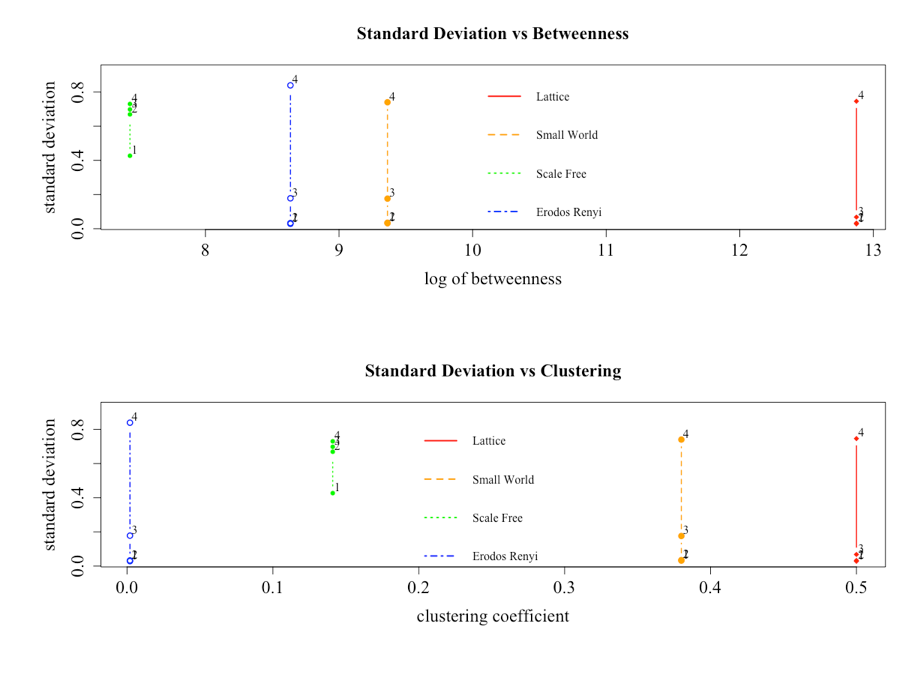
As noted earlier, the creation of bubbles (or volatile behavior) is triggered when the level of trust investors has in the information coming from the network increases beyond a critical point. When this occurs, a positive feedback loop results in mass buying behavior. Alternatively, a collapse occurs when the investors switch camps/herds, almost instantaneously, and begin to sell. As seen in Figure 9, the mechanism that removes the relevance of the network topology is increasing the initial bias towards listening to the network, as dictated by the setting of the c1 variable. The key implication of this is that if investors are highly susceptible to listening to their network rather than other information sources, markets are likely to become more volatile regardless of the network structure, and bubbles result.
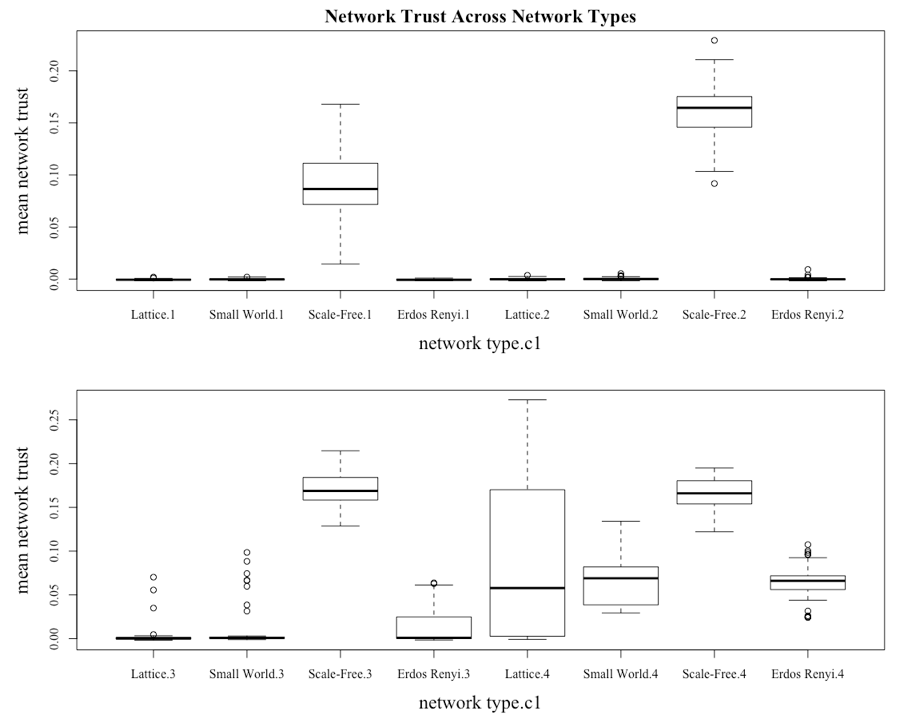
Figure 10 highlights that in line with the price behavior of the asset the different network topologies have very different behavior in terms of the average level of network trust. Consistent with the previous results, the scale-free network is the outlying structure. This is seen with the median of network trust for the scale-free network being both higher and requiring a lower c1 to move it away from 0. It can also be seen that when c1 is set at 4, the median of the network trust is greater than 0 for all the network types, which is consistent with the presence of bubbles under all network types once c1 is increased to 4.
The impact of investors being more susceptible to following their neighbors is illustrated by Thaler (2015), which highlights the observation of Keynes (1937), who had suggested that markets had tended to be more efficient when professional investors using fundamental analysis controlled them. It had been the result of “uneducated” investors, who tended to follow the crowd, entering the market that created the greater volatility. This issue is further compounded when an asset bubble begins to inflate because, as Xiong (2013) points out, more and more less-educated investors are attracted to the market.
Introducing a Multi-Asset Model
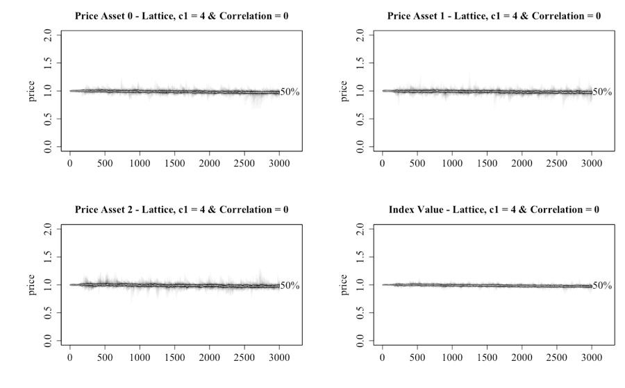
The focus of the paper now moves to understanding how the introduction of multiple assets affects the outcome of the artificial stock market. As discussed earlier, this is considered an important step forward in the field because real-world investors are faced with the dual decision of how to allocate their funds across risky assets as well as between a risk-free asset and risky assets. To understand the impact of introducing multiple assets, experiments utilizing lattice and scale-free networks and using three risky assets were performed. The rationale for this limited subset is that it was these two topologies that produced the greatest difference under the single-asset model. The correlation for the public information of assets, and c1, the initial network information bias, were varied between 0, 0.33, 0.66 and 1 and 1 and 4 respectively. To assist in understanding the dynamics of the system a price-weighted index is also created.
The results of having of 0 correlation between the asset’s public information, and c1 = 4 in a lattice network, are shown in Figure 11. The chart illustrates the individual assets and the index. These settings within the single-asset model were sufficient to see an asset bubble created. However, under the multiple-asset model this does not occur for any of the assets. One can therefore conclude that the need to consider three assets is sufficient to reduce bullish sentiment among the investors, despite the public and private information being generated in a similar manner.
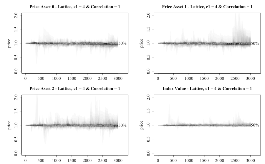
Having established that the introduction of multiple assets with zero correlation delivers a more stable market, Figure 12 illustrates what occurs when the correlation in public information is increased to 1, a scenario that in theory should see greater movement as the assets share the same public information. The result is the appearance of some periods of elevated prices. However, neither the peaks nor the consistency of the appearance of them matches the single-asset case. Another point of note is that while the public information is the same for the three assets, the prices do not move in lockstep as one might expect from a correlated series. This implies that the private information and public information are having significant effects by providing contrary information to the investors. Another possible mechanism is that the trust investors have in public and/or network information may become negative at some point, which will force them into taking a contrary action to what the information suggests.
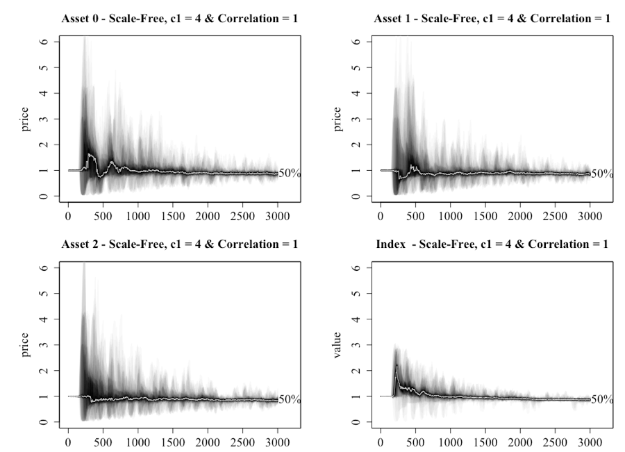
With multiple assets dampening price movements in a lattice network, attention turns to the scale-free network. Figure 13 shows that yet again a market of investors connected by a scale-free network produces very different dynamics, noting that a setting of c1 = 4 allows for a direct comparison with the lattice network charts in Figure 11 and 12. What is seen is that the market consistently enters bubble territory around tick 250, with the market trending back to a median value of 1 but with a high degree of oscillation. When compared to the bottom right of Figure 6 (which provides a comparable chart for a single-asset), the median price of the index is elevated above 1 in the early stages. This occurred because trust in both the public and network sources is systemically higher for the scale-free network.
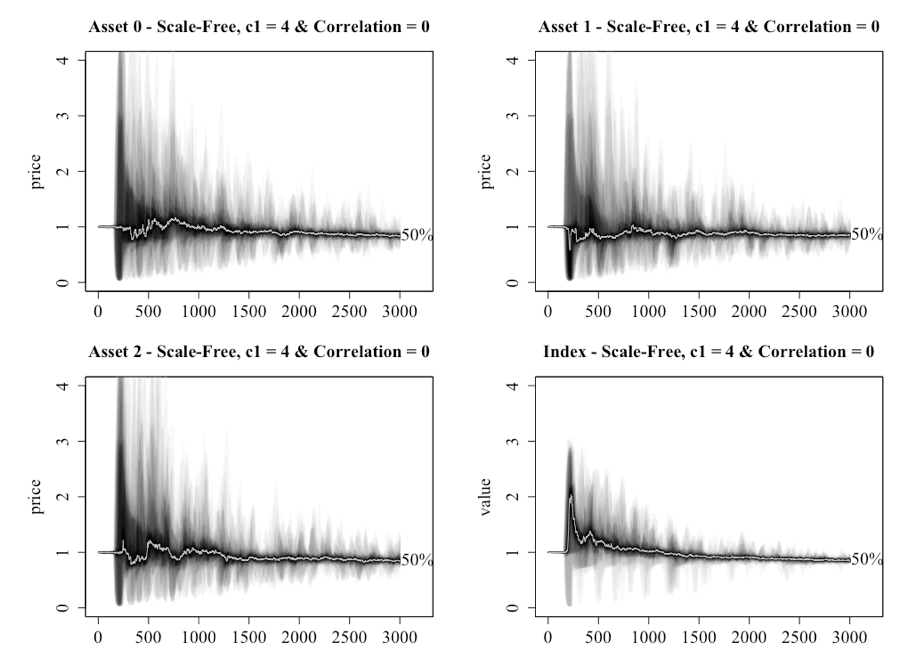
Figure 14 provides an illustration of what occurs when the public information is fully correlated. In the lattice network scenario, as the correlation increased so did the price level and volatility. The opposite appears to occur in the scale-free network as the system appears less volatile. The index still moves away from in the early time periods, but it is not as drastic nor is the volatility as great as when the assets are not correlated.
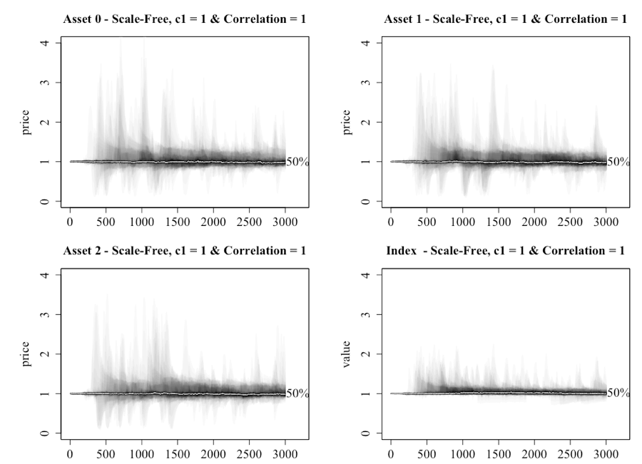
To further illustrate the implications of introducing multiple assets, Figure 15 provides a chart of the scale-free network when c1 is set at 1 and correlation between the public information of the assets is 1. The reader should remember that this was sufficient for an asset bubble to be generated under the single-asset model when using a scale-free network. The results of introducing multiple assets under this scenario are mixed. The extreme price moves do not occur but there is greater movement in the prices than what was seen in the lattice network, despite there being no initial bias to the network information. This result supports the hypothesis that if investors form a network that takes the form of a scale-free network, then the market is more susceptible to extreme price movement despite the public and private information being no different.
Consistent with the presentation of the single-asset model, a clearer picture of the dynamics of the pricing is delivered via the boxplots of the mean of the prices for the assets under the two network structures in Figure 16 and 17. For the lattice network the median price for each of the assets is marginally below 1 across the various settings. This would have arisen because the investors were in general net sellers. Given that the information is generated in the same normally distributed manner, this would have resulted from investors having periods of negative trust in their information sources.
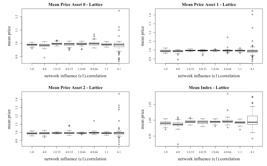
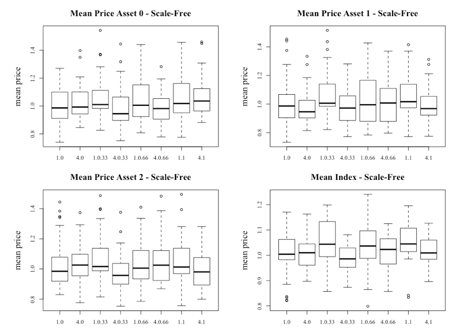
Another result is that the index becomes more volatile when c1 is increased to 4 and as the level of correlation in the public information increases within the subset where c1 = 4. In fact, there is very little volatility within the system until the correlation is increased. However, when comparing the level of volatility as seen in Figure 8, the introduction of multiple assets clearly suppresses the volatility. Figure 17 provides the box plots for the scale-free network, where differences are apparent. The key observation is that there is a larger range of price movement regardless of the level of c1 or correlation when compared to the lattice network.
To provide more conclusive evidence, like the test conducted on the single-asset model, Kruskal-Wallis rank sum tests were conducted on the scenarios summarized in Tables 6 and Table 7. It should be noted that the first table is for the scenario where there is no initial bias to network information (c1 = 1) and the second table shows the results from c1 = 4.
| Correlation | Average | p-value | ||||
| Network | 0 | 0.33 | 0.66 | 1 | ||
| Lattice | 0.990 | 0.995 | 0.994 | 0.992 | 0.993 | (e) <0.01 |
| Scale-free | 1.007 | 1.061 | 1.038 | 1.056 | 1.041 | (e) <0.01 |
| Average | 0.998 | 1.028 | 1.017 | 1.038 | 1.020 | (b) <0.01 |
| p-value | <0.01 | <0.01 | <0.01 | <0.01 | a<0.01 | |
From the data provided in Table 6, the null hypothesis that there is no difference in the price for two networks for a given level of correlation can be rejected (see (a) in Table 6), implying yet again that the network topology that investors form is important. The null hypothesis that there is no difference in the mean price when varying the correlation of the public information across the different networks is also rejected (see (b) in Table 6). The interpretation is that in the multi-asset model the correlation between the public information of the assets does impact the price.
| Correlation | Average | p-value | ||||
| Network | 0 | 0.33 | 0.66 | 1 | ||
| Lattice | 0.986 | 0.994 | 0.998 | 1.002 | 0.995 | (e) <0.01 |
| Scale-free | 1.008 | 0.984 | 1.015 | 1.105 | 1.028 | (e) <0.035 |
| Average | 0.997 | 0.989 | 1.001 | 1.008 | 0.999 | (d) 0.024 |
| p-value | 0.024 | 0.298 | 0.110 | 0.108 | (c)<0.01 | |
Conducting the same hypothesis tests as above, under the scenario when c1 = 4, produces similar results (see (c) and (d) in Table 7). Both tables show that increasing the correlation results in the mean price being statistically different (see (e) in Table 7). With the differences between the single-and multi-asset model, and within the multi-asset model (depending on the level of c1), established, the question turns to understanding why these differences occur. From previous analysis, it is known that the level of trust for the various information sources will be an important source of variation. Boxplots of the average network trust and standard deviations are shown in Figure 18. Consistent with the single asset model, the level and the variability in network trust increases when c1 is increased to 4 for the lattice network. The increased network trust again results in the formation of herds, with the price increasing above and below what would be deemed the fundamental price of the asset. The impact of increasing the correlation of the assets becomes apparent when c1 = 4 and the correlation is at least 0.66.
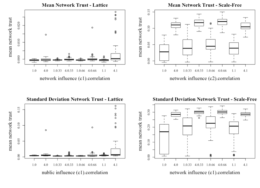
The network trust dynamics are very different under the scale-free network, with two key observations. The first is that the general level of trust within the network is much higher than in the lattice network, with the higher trust recorded when there is an initial bias to network information (c1 = 4). The other observation is that the range of network trust varies greatly based on the level of initial bias to network information (c1 = 4). When c1 = 1, the average level of trust is lower but the range is much greater than when c1 = 4. This point is further reinforced with the bottom right chart in Figure 18, which illustrates the standard deviation of the network trust. The rationale for this result is that without the initial bias to the network information, investors struggle to build and maintain their trust in the information from their neighbors. However, given the dynamics of the scale-free network over the other networks, investors are still able to generate sufficient trust to generate evaluated returns and excessive volatility, again providing evidence that if investors do form a scale-free network, market returns will not be normally distributed in the manner suggested by the EMH.
Discussion and Conclusion
From the various experiments performed in this paper, it is apparent that the network investors form is an important factor in understanding how and why financial markets operate as they do. However, it is also apparent that the outcome of an artificial stock market is very different once investors consider multiple assets.
With regards to the different network topologies it is evident that the different networks had very different characteristics when the c1 variable was set at 1. The first question to come from this is: what is the network structure that the actual market takes? This is not an easy question to answer, given that there are over 10 million investors in the US stock markets (Ozsoylev & Walden 2011). In addition, will this network remain static or does it change over time? Again, this is a very difficult question to answer. However, from the results, all is not lost because there is significant evidence that a bubble will form when investors have formed a scale-free network, regardless of any initial bias to any of the information sources. This outcome is important because researchers can focus on understanding the hubs that exist in financial markets. Examples of hubs include: rating agencies, brokers, large pension funds, and renowned stock pickers such as Warren Buffet. The case can easily be made that if these hubs became correlated then the rest of the investing universe would have little choice but to follow.
Regarding the implications of investors having a higher initial bias towards the actions of their neighbors, Harras and Sornette (2011) cover this extensively. However, this paper made the finding that the network topology becomes a redundant issue at a certain point. The implication stemming from this is the importance of the mindset of the investors entering the market. If new investors are attracted to the market because of a period of abnormally higher returns, they will look to join the herd rather than take the time to undertake fundamental analysis of the markets. Reading The First Crash: Lessons from the South Sea Bubble (Dale 2004), one can see that this behavior is not beyond investors.
In terms of the multi-asset model, the first implication is that for the general ABM community the bar should be moved from producing single risky asset models to multi-asset models. The rationale is that it provides a closer fit to the real-world decisions facing investors, and the effect of multiple assets is sufficient to alter the dynamics of the market. The second implication is that by adjusting, by a certain degree, the correlation between the assets, the behavior is again different. Therefore, further work can investigate how and why the correlation between assets increases in periods of excess volatility.
For the model presented in this paper, there is ample potential to expand the model by introducing greater network dynamics. One such extension would see investors look to disconnect with existing neighbors that they lose trust in, before looking for better-performing investors in the population. Intuition suggests that this process has the potential to see any network structure transform into a scale-free network, as investors gravitate towards the better-performing investor, with a herd and bubble resulting. Another extension would consider the implication of introducing directed links. The current model sees information flow in both directions between neighbors. However, in the real-world information may flow only in one direction due to the nature of the relationship between neighbors or the fact that you do not always listen to someone who listens to you.
Adding dynamic elements to the investors, including their risk aversion and investment threshold, is another field of potential inquiry. In a similar manner to Takahashi and Terano (2003), this extension will allow much of what behavioral finance has put forward with regards to how investors behave as their confidence and returns increase and decrease to be integrated into the model. This paper along with the recommended extensions lays the foundations to better inform regulators and investors so that the instances of inefficient behavior that have been experienced throughout the history of financial markets can be minimized.
Acknowledgements
The author would like to thank the anonymous reviewers for providing valuable comments and suggestions to improve the quality of the paper. Publication of this article was funded in part by the George Mason University Libraries Open Access Publishing Fund. I would also like to thank; George Mason University for providing funding to me through the Presidential Scholarship program, my advisor Prof. Rob Axtell and Prof. Andrew Crooks, for providing insight and guidance in the preparation of this paper.Appendix
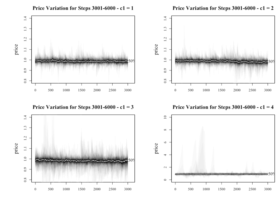
As mentioned in the body of the paper, it is worth considering the behavior of the system pre-and post-bubble. To achieve this the model was run to 6,000 steps using the lattice topology with the results split into the steps 0-3000 and 3,001-6000. Figure 19 presents the results of the first 3,000 steps, with the results consistent with the what was reported earlier in the paper.
The results of the latter half of the runs are provided in Figure 20. The points of notice from the graphs are; bubbles still appear beyond 3,000 steps because of agents taking longer to generate the positive feedback loop that results in the formation of the bubble, and the series with higher levels of c1 (3 or 4), generates higher volatility.
The observation that higher levels of c1 results in higher variability in price, regardless of whether it is the first 3,000 steps or the second, is confirmed in Figure 21. Figure 21 provides the boxplots for the 60 runs, and illustrates that while there is higher variability with a higher level of c1, the difference is not as great for the sample containing steps 3,001 to 6,000.
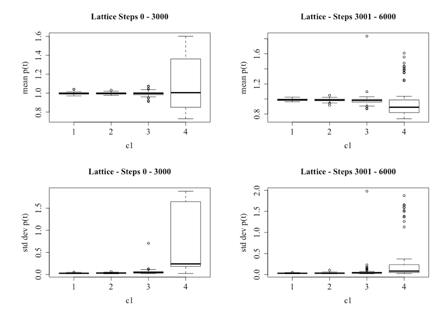
In a manner consistent with the Tables 4 and 5, Table 8 provides the mean and standard deviation for the price series, for differing levels of c1 for the first 3,000 steps and the last 3,000. The main finding being that the volatility of the systems, as given by the standard deviation, remain statistically different for varying levels of c1, regardless of which sample set is used.
| Network Influence c1ij | Average | p-value | |||||
| Network | 1 | 2 | 3 | 4 | |||
| Mean | Lattice (0 -3000) | 0.996 | 0.996 | 0.995 | 1.103 | 1.023 | 0.827 |
| Lattice (3001-6000) | 0.988 | 0.987 | 0.991 | 0.976 | 0.985 | <0.01 | |
| Standard Deviation | Lattice (0 -3000) | 0.030 | 0.033 | 0.061 | 0.806 | 0.233 | <0.01 |
| Lattice (3001-6000) | 0.031 | 0.035 | 0.086 | 0.376 | 0.132 | <0.01 | |
References
ABEL, G. (2015). fanplot: An R Package for Visualising Sequential Distributions. The R Journal, 7(2), 15–23.
ALBERT, R., Jeong, H., & Barabási, A.-L. (2000). Error and Attack Tolerance of Complex Networks. Nature, 406(6794), 378–382.
BARABÁSI, A.-L., & Albert, R. (1999). Emergence of Scaling in Random Networks. Science, 286(5439), 509–512. [doi:10.1126/science.286.5439.509 ]
BOLLERSLEV, T., Engle, R. F., & Nelson, D. B. (1994). 'ARCH models.' (Chapter 49) In Handbook of Econometrics, Vol. 4, 2959–3038.
CALLAWAY, D. S., Newman, M. E. J., Strogatz, S. H., & Watts, D. J. (2000). Network Robustness and Fragility: Percolation on Random Graphs. Physical Review Letters, 85(25), 5468–5471. [doi:10.1103/PhysRevLett.85.5468 ]
CONT, R. (2007). 'Volatility Clustering in Financial Markets: Empirical Facts and Agent-Based Models.' In Teyssière G., Kirman A.P. (eds) Long Memory in Economics. Berlin, Heidelberg: Springer, 289-309.
CONWAY, E. (2009). IMF Puts Total Cost of Crisis at £7.1 trillion. The Telegraph. London.
DALE, R. (2004). The First Crash: Lessons from the South Sea Bubble. Princeton, NJ: Princeton University Press.
ERDŐS, P., & Rényi, A. (1960). On the Evolution of Random Graphs. Publication of The Mathematical Institute of the Hungarian Academy of Sciences, 5(1), 17–61.
FAMA, E. F. (1970). Efficient Capital Markets: A Review of Theory and Empirical Work. The Journal of Finance, 25(2), 383–417.
FARMER, J. D., Gallegati, M., Hommes, C., Kirman, A., Ormerod, P., Cincotti, S., Sánchez, A., & Helbing, D. (2012). A Complex Systems Approach to Constructing Better Models for Managing Financial Markets and the Economy. The European Physical Journal Special Topics, 214(1), 295–324. [doi:10.1140/epjst/e2012-01696-9 ]
GREBEL, T., & Merey, E. (2009). Industrial Dynamics and Financial Markets. Journal of Artificial Societies and Social Simulation, 12(1), 12: https://www.jasss.org/12/1/12.html.
GUPTA, N., Hauser, R., & Johnson, N. F. (2005). Using Artificial Market Models to Forecast Financial Time-Series. arXiv Preprint Physics/0506134.
HAMILL, L., & Gilbert, G. N. (2016). Agent-based modelling in economics. Chichester, UK; Hoboken, NJ: John Wiley & Sons.
HARRAS, G., & Sornette, D. (2011). How to Grow a Bubble: A Model of Myopic Adapting Agents. Journal of Economic Behavior & Organization, 80(1), 137–152. [doi:10.1016/j.jebo.2011.03.003 ]
HOFFMANN, A. O., Jager, W., & Von Eije, J. H. (2007). Social Simulation of Stock Markets: Taking It to the Next Level. Journal of Artificial Societies and Social Simulation, 10(2), 7: https://www.jasss.org/10/2/7.html.
HONG, H., Kubik, J. D., & Stein, J. C. (2005). Thy Neighbor’s Portfolio: Word-of-Mouth Effects in the Holdings and Trades of Money Managers. The Journal of Finance, 60(6), 2801–2824. [doi:10.1111/j.1540-6261.2005.00817.x ]
JANSSEN, M. A. (2017). The Practice of Archiving Model Code of Agent-Based Models. Journal of Artificial Societies and Social Simulation, 20(1), 2: https://www.jasss.org/20/1/2.html. [doi:10.18564/jasss.3317 ]
JOHNSON, N. F., Jefferies, P., & Hui, P. M. (2003). Financial Market Complexity. Oxford; New York: Oxford University Press. [doi:10.1093/acprof:oso/9780198526650.001.0001 ]
KEYNES, J. M. (1937). The General Theory of Employment. The Quarterly Journal of Economics, 51(2), 209–223.
KINDLEBERGER, C. P., & Aliber, R. Z. (2011). Manias, Panics and Crashes: A History of Financial Crises. (6th ed.) Basingstoke: Palgrave Macmillan.
LEBARON, B. (2006). 'Agent-based Computational Finance.' In Testfatsion, L. & Judd, KL (eds), Handbook of Computational Economics, Vol. 2. Amsterdam: North Holland, pp. 1187–1233.
LUX, T. (2016). Financial Power Laws: Empirical Evidence, Models, and Mechanism. Chaos, Solitons & Fractals, 88, 3-18. [doi:10.1016/j.chaos.2016.01.020 ]
MANDELBROT, B. (1963). The Variation of Certain Speculative Prices. The Journal of Business, 36(4), 394-419.
OZSOYLEV, H. N., & Walden, J. (2011). Asset Pricing in Large Information Networks. Journal of Economic Theory, 146(6), 2252–2280. [doi:10.1016/j.jet.2011.10.003 ]
OZSOYLEV, H. N., Walden, J., Yavuz, M. D. & Bildik, R. (2014). Investor Networks in the Stock Market. Review of Financial Studies, 27(5), 1323–1366.
PANCHENKO, V., Gerasymchuk, S., & Pavlov, O. V. (2013). Asset Price Dynamics with Heterogeneous Beliefs and Local Network Interactions. Journal of Economic Dynamics and Control, 37(12), 2623–2642. [doi:10.1016/j.jedc.2013.06.015 ]
R CORE TEAM. (2015). R: A Language and Environment for Statistical Computing. Vienna, Austria: R Foundation for Statistical Computing: https://www.R-project.org/.
SANTOS, F. C., & Pacheco, J. M. (2005). Scale-Free Networks Provide a Unifying Framework for the Emergence of Cooperation. Physical Review Letters, 95(9). 098104. [doi:10.1103/PhysRevLett.95.098104 ]
SHILLER, R. J., & Pound, J. (1989). Survey Evidence on Diffusion of Interest and Information Among Investors. Journal of Economic Behavior & Organization, 12(1), 47–66.
SORNETTE, D. (2014). Physics and Financial Economics (1776–2014): Puzzles, Ising and Agent-Based Models. Reports on Progress in Physics, 77(6), 62001. [doi:10.1088/0034-4885/77/6/062001 ]
SQUAZZONI, F. (2010). The impact of agent-based models in the social sciences after 15 years of incursions. History of Economic Ideas, 18(2), 197–233.
TAKAHASHI, H., & Terano, T. (2003). Agent-Based Approach to Investors’ Behavior and Asset Price Fluctuation in Financial Markets. Journal of Artificial Societies and Social Simulation, 6(3), 3: https://www.jasss.org/6/3/3.html.
WALDEN, J. (2014). Trading, Profits, and Volatility in a Dynamic Information Network Model. SSRN Electronic Journal.
THALER, R. (2015, July 10). Keynes’s "Beauty Contest." Financial Times: https://www.ft.com/content/6149527a-25b8-11e5-bd83-71cb60e8f08c.
WATTS, D. J., & Strogatz, S. H. (1998). Collective Dynamics of "Small-World" Networks. Nature, 393(6684), 440-442.
WILENSKY, U. (1999). Netlogo. Northernwestern University. Evanston, IL: Center for Connected Learning and Computer-Based Modeling: http://ccl.northernwestern.edu/netlogo.
XIONG, W. (2013). Bubbles, Crises, and Heterogeneous Beliefs (No. w18905). Cambridge, MA: National Bureau of Economic Research.