
Introduction
Extortion has been defined as a kind of tax imposed by organized crime on firms established in a region, sometimes in exchange of protection against other criminals (Astarita et al. 2018). The tax, paid in cash, goods, or services, is known as pizzo in Italy or piso in some Latin American countries. Such criminal activity is present in many economies (Konrad & Skaperdas 1998), hence the interest in studying its macroeconomic effects and the microfoundations that generate them. To do this, we propose a methodology consisting in simulating a healthy economy and then introducing extortion at different levels of activity, comparing subsequently the macroeconomic signals produced in both situations.
Our approach is justified given the hidden nature of extortion that makes it difficult to determine both its extent, and its diverse and complex effect on society (Troitzsch 2017); either at an individual or collective level (Gutierrez-Garcia et al. 2013). In spite of the lack of precise measures and the fact that numbers vary worldwide, the following examples illustrate its magnitude: Most Chinese business owners in New York have had meetings with gang members who approached them for money, goods or services, and most of them seem to have paid (Venkatesh & Chin 1997); It is estimated that up to 80% of firms could have paid some type of extortion (Anzola et al. 2016; Gambetta 1996); The hidden nature of extortion in Mexico evidences a high percentage of 97.8%, i.e., for every 22 reported extortion crimes, there are 978 not reported (Morales et al. 2015).
The difficulties of getting real data to analyze the macroeconomic effect of extortion are evident. We alternatively propose to cope with the lack of data by modeling and simulating extortion in terms of the behavior of the agents involved in a simulated economy, i.e., focusing on the underlying microfoundations and analyzing the emerging macroeconomic signals. As in many other domains (Parunak et al. 1998), two main approaches can be followed when it comes to model an economy (De Grauwe 2010): the classical equation-based approach and the agent-based approach (bottom-up).
The central statement of equation-based economic modeling establishes that general equilibrium on all markets derives from the interaction between supply and demand. An important characteristic of these models is the market clearing condition (Walrasian auctioneer), which is given by a central authority that proposes a set of prices, determines an excess of demand at these prices and adjusts them to their equilibrium values.
One of the main limitations of equation-based modeling approach is the assumption of equilibrium, since it can arguably be too simplistic for capturing the complexity of economic processes over time. The so-called Dynamic Stochastic General Equilibrium (DSGE) model has largely prevailed in the economic literature (Christiano et al. 2018; Kydland & Prescott 1982; Woodford 2003). In general a DSGE model is a non-linear set of stochastic difference equations. These equations are the necessary conditions of the optimization problems. Tackling directly the stochastic non-linear equations is very difficult, so the original problem is replaced by an approximation. Depending on what you ask to the model, this approximation will be more or less accurate. DGSE is just able to pick up small fluctuations around a stationary state, even though external shocks are used to get it out of equilibrium. These sort of models behave well when there are no disturbances, but predict poorly when risk and uncertainty come into play (Fagiolo & Roventini 2017; Stiglitz 2017).
On the other hand, the bottom-up approach conceives models as composed of autonomous agents exhibiting bounded rationality, i.e., individuals with a purposeful behavior guided by some measure, e.g., higher salary offered by firms, lower interest rate of banks or better leverage of firms; but that are subject to limited deliberative resources, e.g., lack of information or time for taking decisions. Two important features of this kind of models are heterogeneity, i.e., each agent has its own attributes and behavioral rules; and emergency, i.e., the effect of the diversity and the interactions among the agents can be observed in the behavior of the system as a whole (Macal & North 2010).
Bottom-up models do not make assumptions about the efficiency of markets, neither about the existence of an equilibrium, so they can absorb the tensions or disturbances generated in periods of crisis through the emerging behavior resulting from the interactions among the agents. Furthermore, these models are non-linear in nature, which implies that the generated effects do not have to be proportional to their causes. This allows to identify such causes in areas that in principle are not related to the effects. In some models, the effects can be of a magnitude much greater than the causes that provoke them while in others the effects dissipate in a conventional manner.
All this considered, the Bottom-up Adaptive Macroeconomics (BAM) model (Delli Gatti et al. 2011) has been adopted as the mechanism to generate the baseline economy for the simulation of extortion. The BAM model has been widely documented and it has been described using the ODD protocol (Platas-López et al. 2019). An open-source implementation of the model has been released and used for validation with respect to the expected wealth distribution, while studying the effect of market size and the presence of shocks in wages, prices or interest rates (Platas-López et al. 2020).
BAMERS (BAM under Extortion Racket Systems) is the agent-based model proposed in this work to study the effect of extortion on macroeconomic signals. The model has a double influence: (i) for the sake of simplicity, it is assumed that the economic pressure and social status might move poor workers to become extortionists (Abrahamsen 1949); and (ii) parametrization and initialization of extortion is done by following the outcomes of the GLODERS project (Elsenbroich et al. 2016). Therefore, BAMERS extends the BAM model by allowing a certain number of poor, unemployed workers to become extortionists asking firms to pay the pizzo. Firms, in turn, have the choice to pay or to refuse and denounce. Extortionists have a chance of being captured and punished, a simplified way of modeling the effectiveness of police and justice. Money recovered from extortionists imprisoned is distributed among the denouncing firms. On the other hand, extortionists that escape the law punish the firms that denounced them.
The interaction of the extortionists with other agents in the model induces changes in macroeconomic signals such as inflation, unemployment, and Gross Domestic Product (GDP) measured in monetary units. Comparing these signals with those produced by the baseline economy offers clues about the macroeconomic effect of extortion. In general, the outputs exhibit a generic phase transition from the baseline economy to a statistically different one. In particular, our results show an inverse relationship between extortion and the real GDP, indicating that extortion has a negative effect on the aggregate supply. All in all, the proposed approach seems adequate and necessary to study the economic nature of extortion.
The rest of the paper is organized as follows. In Section 2, introduces related work. First, the BAM model is briefly described, highlighting the properties that make it an adequate baseline economy for studying the macroeconomic effect of extortion. For the sake of replicability, the ODD description of the BAM model is included in the Appendix. Then, some works related to the dynamics of extortion are discussed, including an equation-based approach for comparison. Section 3 introduces the BAMERS model, adopting the ODD protocol. Section 4,defines and justifies our methodological approach, including the experimental setup, the variables of interest, and the different tests and analyses performed. Results are presented in Section 5, including an analysis of the population dynamic under extortion; a robustness analysis of the model parameters; and the macroeconomic effect of extortion on consumption, Gini index, GDP, inflation, unemployment rate and wealth distribution. Section 6 concludes and discusses future work.
Related Work
This section introduces the Bottom-up Adaptive Macroeconomic model (Delli Gatti et al. 2011), adopted to our baseline simulated economy. It is shown that this model reproduces desired stylized facts while exhibiting good sensibility to changes in its parameter values. Then, recent works related to the dynamics of extortion are briefly reviewed, focusing on the normative and behavioral aspects of extorters and the effect of extortion on wealth distribution. An equation-based approach to the study of the effect of extortion, among other criminal activity, on economy is also reviewed for the sake of comparison.
The Bottom-up Adaptive Macroeconomic (BAM) model
As Alves-Furtado & Eberhardt (2016) point out, one of the main problems faced in macroeconomic analysis is the choice of a base model, since some of them are too generic while others are specialized in particular markets, e.g., energy or labor. Dawid & Delli Gatti (2018) make a classification of macroeconomic agent-based models according to their size and distinguish between large, medium and small. Small models are characterized by having only two types of agents, households and firms, interacting in two markets, consumer goods and labor. Large models present at least three types of agents and at least five markets.
The BAM model (Figure 1) is a generic, medium-sized, economic model that belongs to the Complex Adaptive Trivial Systems (CATS) family of models reviewed by Dawid & Delli Gatti (2018); being one of the best documented, more extended, and widely used models among this family (Delli Gatti & Desiderio 2015; Gualdi et al. 2015; Klimek et al. 2015). The model is composed by three types of agents:
- Households, representing the point of consumption and labor force.
- Firms, representing the transformation of work in goods and / or services.
- Banks, that provide liquidity to firms if necessary.
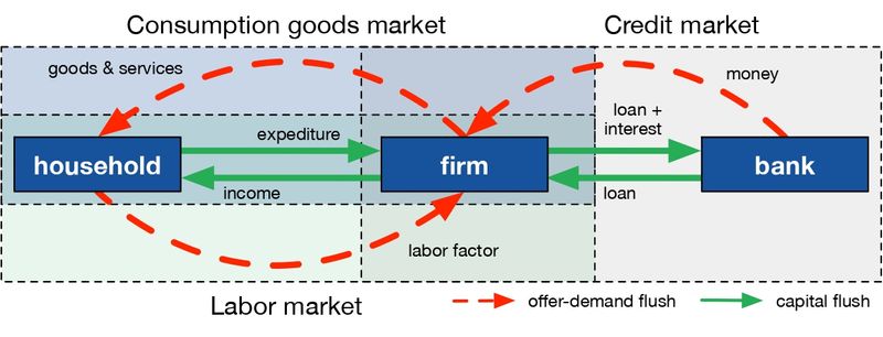
A large number of these agents operate adaptively in three totally decentralized and interconnected markets:
- A labor market in which each household offers an inelastic unit of work per period, while firms demand depending on their production plans;
- A perishable consumer goods market, in which households spend all or part of their wealth and firms offer goods at different prices; and
- A credit market in which firms demand money if their resources are insufficient to cover their production expenses, and banks offer money at different interest rates.
Opportunities for exchange in these markets are discovered through a sequential process characterized by optimization, namely: maximizing wages, minimizing the price of goods consumed, and minimizing the price of money (interest rate). Firms can modify prices and production given the signals of the inventory and the market price. The schedule of a simulation step, representing a month in the BAM model, is as follows:
- Firms calculate production based on expected demand.
- A decentralized labor market opens.
- A) A decentralized credit market opens. B) Credit market closes. C) Labor market closes.
- Firms produce.
- A) Goods market opens. B) Goods market closes.
- Firms pay loans and dividends.
- Firms and banks survive or die.
- Bankrupt firms and banks are replaced.
Our implementation of the BAM model1 produces macroeconomic signals of interest such as inflation, unemployment, wealth or production, among others. The default parameter settings generate an artificial stable economy with unemployment rate around 10% and moderate inflation in the range of 1% to 6%. These numbers are similar to the data for the period 2014–2018 reported by the (World Bank 2019b, 2019a), in which the average unemployment rate across countries was 8.22% and the average annual inflation was 4.43%. For a full description of the BAM model and validation results see Platas-López et al. (2019) and Platas-López et al. (2020). A more concise description using the ODD protocol is included in the Appendix.
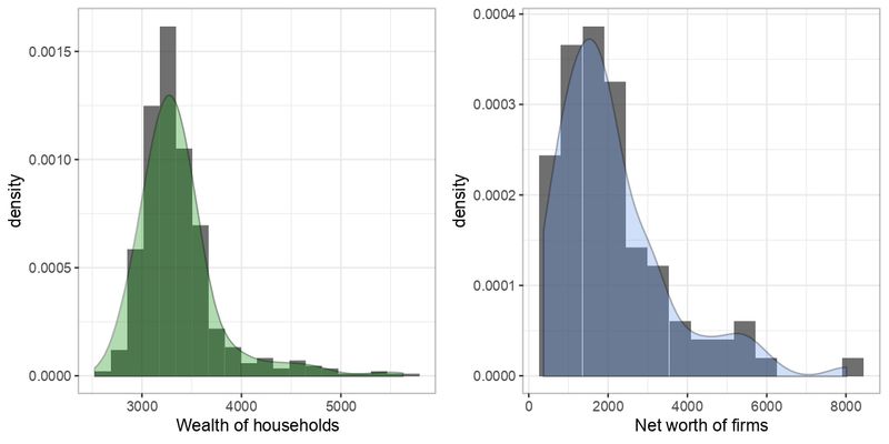
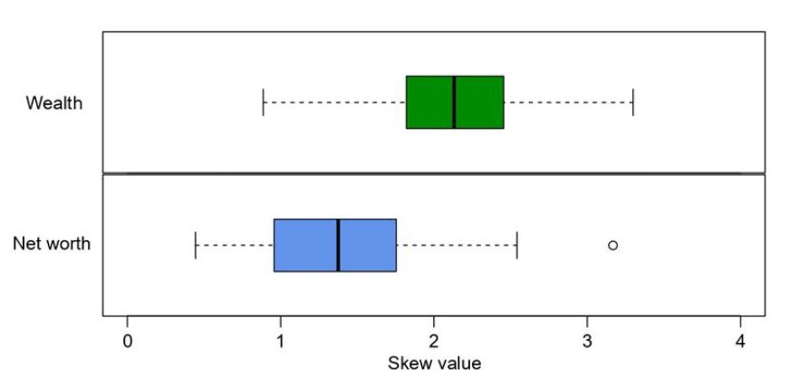
At the micro level, the model reproduces stylized facts in the distribution of agent’s state variables (Delli Gatti et al. 2011). For example, the wealth of households and the net worth of firms are characterized by a positive skew as shown in Figure 2. Following Joanes & Gill (1998), we calculated the skewness of wealth and net worth distributions over 100 independent runs. Both distributions are characterized by a positive skew \(> 1\), as shown in Figure 3, confirming an expected situation in which few agents are becoming rich.
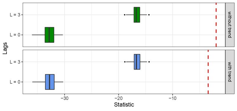
At the macro level, it is assumed that an economy is characterized in the long run by a balanced growth or, in other words, that series do not have a time dependent structure, e.g., the growth rate of GDP is mean stationary (Evans 2000). To verify the stationarity of the serie, we used Dickey Fuller Test, which is one of the most widely used statistic test. It uses an auto-regressive model and optimizes an information criterion across multiple different lag values (Harris 1992). By applying this test with and without trend for zero and 3 lags on the last 500 time steps of GDP growth for 100 independent runs, with \(\alpha=0.05\), it is possible to reject the null hypothesis of non-stationarity if the t-statistic value is less (more negative) than the critical values (respectively, -3.42 and -1.95 for the test with and without trend). As shown in Figure 4, GDP growth rate series are mean stationary since this stylized fact is fulfilled for all independent runs.
These results endorse the choice of BAM as a baseline economic model to study the effect of extortion on the macroeconomic signals produced by this artificial economy.
The dynamics of extortion
Different agent-based models of extortion have been proposed in literature. Extortion can be carried out by individuals, but it is more often executed by organized groups configuring extortion racket systems. Even though, for the sake of simplicity literature models that analyze the relationship between the mafia and society decide to treat the mafia as individual agents (Elsenbroich & Badham 2016; Nardin et al. 2016; Troitzsch 2014). The outcomes of the European project GLODERS 2 (Global Dynamics of Extortion Racket Systems), resulting in a large corpus describing the behavior of extortion racket systems (Andrighetto, Brandts, et al. 2016; La Spina et al. 2014; Nardin et al. 2017), are very useful to understand the microfoundations of extortion, as well as the normative, legal and social aspects that help to understand and fight against it (Andrighetto, Giardini, et al. 2016; Lotzmann et al. 2013; Nardin et al. 2016; Realpe-Gómez et al. 2018; Villatoro et al. 2015). Other efforts focused on the immediate effect of crime from the criminologist perspective can be found in the work by Gutierrez-Garcia et al. (2013).
Unfortunately, most of these works do not adopt a macroeconomic perspective. An exception is Troitzsch (2014), who analyzes extortionist groups by focusing on three aspects: the effect on wealth distributions of firms and criminals; the change in the propensity of firms to contribute to the fight depending on the attitude of the public towards extortionist groups; and the study of individual agent behaviors showing the greatest effect on society as a whole. On the first aspect, which is in fact related to the scope of this work, Troitzsch concludes that:
The distribution of the overall economic success of the extortionists is extremely skewed to the left which shows that for a majority of input parameter combinations the success of extortionists is low, the main determinant for low success being the prosecution propensity.Troitzsch’s model is a good starting point to analyze the effects of extortion on other macroeconomic signals. In order to achieve this goal, our model does not abstract the market of goods and labor to observe the emerging behavior on unemployment, inflation, and production. Table 1 summarizes a selection of extortion models that were taken into consideration while creating the model proposed in this work.
| Reference | Extortion | Payment | Capture | Refund | |
| Troitzsch (2014) | To the nearest reachable firm within its territory. Successful extortionist will then protect the shop against the rival extortionists. | If a firm cooperates, the pizzo is a proportion (low 25%, high 50%) of the period’s income. If a firm refuses to pay the pizzo, the punishment may be a proportion (low 25%, high 50%) of all assets. | Police captures with a probability of success (30%). Captured extortionists are jailed for 6 periods (no time scale is given). | All assets are taken from the extortionist and firms are compensated following a first come first served principle. | |
| Elsenbroich & Badham (2016) | Every period, extortionists choose a random firm within its territory, if it has not been extorted, they try to extort it. | The pizzo is constant in 100 units. | Neither capture nor imprisonment is specified. | No refund specified. | |
| Nardin et al. (2016) | Search details are not specified. | The pizzo is a proportion (low 3%, high 10%) of the firm resources. The punishment is a proportion (low 50%, high 75%), which is applied with a probability (low 50%, high 90%). | There is a probability of capture (low 20%, high 80%). Captured extortionists are jailed, the number of periods is not specified. | The victim support fund is made up of a percentage of the mafia’s resources (0% or 50%). | |
| Nardin et al. (2017) | Search repeatedly until a new firm is found. After each attempt there is a probability (10%) of abandoning the search. | The pizzo is a proportion (low 3%, high 10%) of the wage of firm. The punishment is a proportion (low 50%, high 75%, very high 90%) of the wage of firm. | There is a probability of being captured (low 20%, high 80%). Captured extortionists are jailed, the number of periods is random with a normal probability distribution function with mean low 100 (or high 500) and standard deviation low 5 (or high 100). Each period represents a day. | The victim support fund is made up of a percentage of the mafia’s resources (0% or 50%). Firms who have denounced form in a queue, if the fund is sufficient a firm is refunded and returned to the queue. |
Effects of crime on the economy
Although the empirical evidence seems to detect an adverse effect of organized crime in the economy, a theoretical framework to explain all possible ways for organized crime to influence an economy has yet to be developed. Astarita et al. (2018) propose an equation-based model to study the macroeconomic impact of organized crime. They found that some activities, e.g., extortion, illegal trade and corruption, reduce demand by extracting resources from the legal sector, while others can increase demand, e.g., money laundering.
The negative effect of organized crime on the economy comes in three different ways:
- A reduction in productive capital, due to a decrease in domestic savings and foreign investment. In fact, less security in property rights, leads to a poor business environment, discouraging innovation and entrepreneurship.
- The diversion of public resources destined for policies that improve growth, e.g., education and infrastructure, towards policies that guarantee protection against crime.
- A reduction in the labor supply, since people can choose to provide their services in the illegal sector, instead of the legal one.
Demand for illegal goods is a linear function of legal income that depends on three elements:
- The propensity to consume illegal goods through legal disposable income.
- The ability of organized crime to appropriate legal revenues through crimes such as extortion.
- The propensity to consume illegal goods through illegal income.
Astarita et al. (2018) implement the principle of effective demand through a standard neo-Kaleckian investment function, where the investment decision of a firm depends on the level of economic activity. Four types of crime are considered:
- Extortion, a tax normally paid in cash by firms to criminal groups, that pursues several objectives: (i) establish a constant flow of income; (ii) establish a social and economic network that facilitates the infiltration of organized crime in the legal economy; and (iii) reach a monopolistic position in some productive sector.
- Corruption of public officials, allowing for the misappropriation of part of the public resources destined to transfer income, services and infrastructures.
- Trade in illegal goods, mainly drug trafficking, representing the main source of revenue for organized crime and a flight of income from the legal economic system.
- Money laundering, which allows to conceal the illegal origin of criminal profits and transform them into effective purchasing power, that is, into a potential demand for consumption and investment.
The main contribution of the model by Astarita et al. (2018) is that it explains how organized crime differently affects economic activity and growth, also identifying the analytical conditions for a positive or negative effect of crime on the economy. The results for this model use data from the Italian economy and can be taken as a point of comparison for the proposed bottom-up model, regardless of the economic paradigm adopted, Keynesianism or Neoclassic (Palley 1998). Indeed, whereas extortion has a negative effect on demand in the model by Astarita et al. (2018), our model exhibits a negative effect on production.
BAMERS: The BAM under Extortion Racket Systems model
The Bottom-up Adaptive Macroeconomics under Extortion Racket Systems (BAMERS) 3 model extends BAM by introducing extortionists in the system. In what follows, it is described following the ODD protocol (Grimm et al. 2006, 2010).
Overview
Purpose
BAMERS is designed to explore the effect of individual extortion activities in macroeconomic signals like GDP, inflation, unemployment rate, and Gini index.
Entities, state variables, and scales
- Environment. Originally the grid environment where the agents are situated was used exclusively for debug purposes, displaying information useful for validating the behavior of the system, e.g., the number of workers laboring in a firm, their presence when working and buying goods, etc. Beyond this, the BAMERS model uses neighborhood in this space when computing some decisions, even when such relation has not geographical meaning, i.e., neighbors are not assumed to be geographically closed together.
- State variables. Firms and workers, as originally defined in the BAM model, are extended with the variables shown in Table 2 for registering the effect of extortion activities. Unemployed workers may become extortionists and keep a list of firms to extort and possibly punish. When captured, an extortionist will be in jail a given number of periods (time-in-jail). Firms register if they are being extorted and keep record of the amount of wealth they paid as pizzo or punishment.
- Scales. Time is represented in discrete periods, each step representing a month.
| Firm | Worker | |||
| Attribute | Type | Attribute | Type | |
| being-extorted? | Bool | extortionist? | Bool | |
| amount-of-pizzo | Float | firms-to-extort | AgSet | |
| amount-of-punish | Float | firms-to-punish | AgSet | |
| time-in-jail | Int | |||
Process overview and scheduling
Extortion in the BAMERS model occurs after closing the goods market and before firms pay loans and dividends, i.e., in between steps 5 and 6 of the BAM model schedule. Events occurs into one monthly period. For the purposes of the paper this is an allowable simplification. The new steps added to the schedule are as follows:
- A) Goods market opens. B) Good market closes.
- Unemployed poor workers decide whether to become extortionists or not.
- Extortionists look for firms to extort.
- Firms pay the pizzo or refuse to pay and denounce.
- Extortionists punish firms that refused to pay or, when captured, they go to jail and lose their wealth.
- Prisoners that have served their time in prison are released as regular unemployed workers.
- Firms will pay loans and dividends.
Design concepts
Basic Principles
Economic pressure and socioeconomic status induce a process of decision making on how to respond to basic needs, even considering the idea of becoming criminals. Abrahamsen (1949 p. 140) wrote about this:
There are a few questions that are frequently asked in regard to our findings that family tension is the basic cause of criminal behavior. The first has to do with economics. It is reasonable to assume, intellectually speaking, that when one is without what is necessary for subsistence and cannot get it, he will simply take it for himself and his loved ones. This is instinctive, and it has to do with self-preservation.
Adaptation
Following the basic principle enunciated above, every time the goods market closes, unemployed workers belonging to the poorest quartile in the population decide as to whether they will become extortionists or not with a propensity \(\epsilon\). The propensity to become a criminal is orthogonal to any other variable, e.g., the probability of being imprisoned \(\lambda\). This enables a controlled complete parameter exploration to evaluate the macroeconomic effect of extortion. When \(\epsilon\) is equal to zero, our model corresponds to the baseline macroeconomic model without extortion, i.e., the BAM model.
Sensing
Firms can observe a given number of firms to know if they are paying for pizzo or not.
Interaction
Interaction happens when an extortionist finds a firm and asks for the payment of pizzo. Firms can in turn accept, or refuse to pay and denounce.
Stochasticity
Processes exhibiting randomness include becoming an extortionist, being imprisoned, and trying to extort a firm. The search for potential firms to extort is also stochastic.
Details
Initialization
Table 3 shows the default parameter initialization for the BAMERS model. Parameter values are influenced by the work of GLODERS (Elsenbroich & Badham 2016; Nardin et al. 2016, 2017; Troitzsch 2014).
| Parameter | Value | |
|---|---|---|
| \(\epsilon\) | Propensity to become an extortionist | 20% |
| \(\lambda\) | Probability of being imprisoned | 30% |
| \(R_t\) | Rejection threshold | 15% |
| \(X\) | Number of attempts to extort a new firm | 1 |
| \(CF\) | Number of observable closest firms | 3 |
| \(Pi\) | Proportion of net worth asked as pizzo | 20% |
| \(Pu\) | Proportion of net worth taken as punish | 30% |
| \(C_m\) | Proportion of wealth as confiscated money | 50% |
| \(T_j\) | Number of time periods in jail | 6 |
Submodels
Here is a description of the use of parameters:
- The number of extortionists in the system may change every time step. Each unemployed worker in the quartile with the lower savings becomes a criminal if the propensity to be an extortionist \(\epsilon\) is greater than a randomly generated value with a uniform distribution between 0 and 100.
- An extortionist has \(X\) attempts to find a new victim. If an extortionist selects a firm that is already being extorted, it is considered as a failed attempt.
- Extortionists choose their victims by searching randomly over all firms.
- Firms can allow the extortion or refuse to pay. A firm refuses to pay the pizzo when the rejection threshold (\(R_t\)) is greater than the expected risk (\(ER\)) , which is calculated as follows:
where, \(CF\) denotes number of observable firms (three by default), i.e., the closest ones; and \(EF\) denotes how many of them are being extorted. This cognitive mechanism is based on the work of Elsenbroich & Badham (2016). \(R_t=0\) makes firms to pay the pizzo at the slightest hint of extortion activity.\[ER = \frac{EF}{CF}\] \[(1)\] - Firms that accept to pay the pizzo are asked for a proportion of their net worth, set by default to \(Pi=20\%\) as suggested by Troitzsch (2014), Nardin et al. (2016) and Nardin et al. (2017).
- Firms that refuse to pay the pizzo always denounce. The probability that an extortionist is imprisoned is set to \(\lambda=30\%\). Imprisoned extortionists stay \(T_j=6\) periods in jail. Additionally, a proportion \(C_m=50\%\) of their wealth is confiscated for supporting the victims of extortion that had denounced. All the previous default parameter values were adopted from the findings by Troitzsch (2014), Nardin et al. (2016) and Nardin et al. (2017).
- Extortionists that are not imprisoned punish the firm that denounced them, if any. The amount of money taken as punishment is a proportion of the net worth of the firm set by default to \(Pu=30\%\).
- Firms who have denounced and were punished receive an equal proportion of the victim support fund raised from 50% of imprisoned extortionists wealth.
- Extortionists who served their sentence become regular workers in the labor market, in the immediate following period.
Methodology
In order to compare the macroeconomic outcome of the simulated economies under different levels of extortion, a set of scenarios is defined through parametrization. In what follows, we introduce the experimental setup producing these scenarios. Then, we justify the selection of macroeconomic variables used in our analyses. Finally, we describe the tests we performed on the selected variables, mainly: measuring the model robustness to understand what responses are emergent properties of the system and which ones are a direct consequence of the parametrization; and the Cucconi test to identify changes in the distributions of macroeconomic variables.
Experimental setup
We simulate a small baseline economy showing a stable growth and moderated unemployment rate consisting of 100 firms, 500 households and 10 banks, that were initialized as described by Delli Gatti et al. (2011) and implemented following Platas-López et al. (2019).
Extortion is introduced in this economy as described in the previous section. A default scenario is defined initializing the parameters of the BAMERS model as shown in Table 3. Three of them are perturbed to induce different scenarios: The propensity to become an extortionist (\(\epsilon\)) takes percentage values from 0 to 100 in increments of 5; The probability of being imprisoned (\(\lambda\)) is perturbed in the same way; The rejection threshold (\(R_t\)) differentiates the propensity to denounce of the firms, given the submodel for computing the expected risk (submodel 4) and the number of the observable closest firms (\(CF=3\)). When \(R_t=0\) the firms never denounce extortion. For \(0<R_t\leq 33\), the firms denounce if none of the observable firms is under attack, i.e., extorted or punished. For \(33 < R_t \leq 66\) the firms denounce if at most one of the observable firms is under attack. For \(66 < R_t \leq 99\) the firms denounce if at most two of the observable firms is under attack. When \(R_t=100\) the firms always denounce. A low tendency to denounce (\(R_t=15\)) and a moderate one (\(R_t=45\)) are explored here, since higher or lower tendencies seem unrealistic.
All experimental settings and tests were performed over 20 independent runs. Each simulation run represents around 40 years, using a monthly time scale with 1000 periods and discarding the first 500 time steps as burning period. Although the model seems to converge in the first 200 periods, it was decided to discard 300 more periods to guarantee convergence regardless of the parameter settings.
Variables of interest
Different economic paradigms emphasize different macroeconomic variables, e.g., while classical Keynesianism focus on demand, neoclassical economy does on productivity. However, any macroeconomic analysis should consider at least the following three key variables: production, employment and price. We measure these variables using the real GDP, the unemployment rate and inflation, respectively. Since the distribution of wealth is an important component in economic development analysis, the Gini index will also be considered. Finally, the wealth of extortionists and household consumption are also included to be compared with the results by Troitzsch (2014) and Astarita et al. (2018).
GDP is a measure of the value of the output of an economy. The real GDP captures the effect of changes in prices over time, its values being comparable at different times. The unemployment rate is a measure that relates the number of unemployed people to the total amount of available labor force, this excludes people in prison. Inflation is measured by the Consumer Price Index and it is defined as a change in the prices of a basket of goods and services that are typically acquired by a specific group of households. In the BAMERS model, inflation is summed up to the change in the price of the only good produced in monthly periods.
Wealth is composed of the income of workers as well as their savings, inequality in the distribution of wealth among individuals is measured through the Gini Index, which is based on the comparison of cumulative proportions of the population against cumulative proportions of wealth they have, and it ranges between 0 in the case of perfect equality and 1 in the case of perfect inequality. Like regular workers, the wealth of extortionists is made up of their income from extortion and punishment of firms as well as their savings. Finally, household consumption is an aggregate variable that represents the total purchases of goods made by 500 households in the system. At micro level, the marginal propensity to consume \(c\) (defined in App. 1.1.7) reflects the variation in consumption with respect to the variation in income/wealth, the complement representing the marginal propensity to save. The higher the income/wealth the lower the proportion spent on consumption. That is, rich people usually tend to have a lower marginal propensity to consume \(c\) than poor people.
It is important to mention that all the variables related to money (wealth, pizzo, consumption, etc.) will be analyzed with respect to the GDP, so that different scenarios (at different values of \(\epsilon\), \(\lambda\) and \(R_t\)) can be compared appropriately.
Robustness analysis
Robustness analysis examines the effect of varying input parameters on the output of the simulation. High sensitivity to these values suggests that such an effect would be due to parametrization, rather than being an emerging property of the model (Helton 2008). The robustness of the BAMERS model is determined by modifying the probability of becoming an extortionist (\(\epsilon\)) and the probability of being imprisoned (\(\lambda\)), as these are considered to be the most important parameters for this work.
We increase the value of \(\epsilon\) and \(\lambda\) from 0 to 100 in steps of 5 units independently from all other parameters. The output of each setting is then compared with that of the model with all the parameters set to their default values using the A-Test (Vargha & Delaney 2000). This is an effect-magnitude test used to determine if there is any statistically significant difference between simulation responses under different conditions, thus indicating how robust the model is to changes of its parameters and the points at which parameter perturbation results in significant changes in the simulation (Alden et al. 2013).
The A-Test can be applied both to discrete (at least ordinal) and continuous distributions, which makes it applicable to behavioral and social science domains where discrete scales are common. It makes no assumptions of normality or homogeneity of variance, and it is easier to compute than the CL-Test (Vargha & Delaney 2000 p. 102).
We can interpret the result of the A-Test as follows: We have stochastic equality between two populations when \(A_{ij}=A_{ji}=0.5\), where \(A_{ij}\) denotes the comparison of population \(i\) to \(j\). Vargha & Delaney (2000) propose thresholds to interpret the effect size \(\Delta\), i.e., the standardized difference between populations, which are summarized in Table 4.
| \(\Delta\) | A-Test | Difference |
|---|---|---|
| 0.50 | 1.00 | Total |
| 0.21 | 0.71 | Large |
| 0.14 | 0.64 | Medium |
| 0.06 | 0.56 | Small |
| 0.00 | 0.50 | None |
| 0.06 | 0.44 | Small |
| 0.14 | 0.36 | Medium |
| 0.21 | 0.29 | Large |
| 0.50 | 0.00 | Total |
Comparing distributions of macroeconomic signals
Different levels of extortion are expected to produce different macroeconomic signals in the simulation. Comparing these outputs poses the problem of comparing distributions of variables of interest in which normality or any other property cannot be guaranteed. Since both mean and variance may differ between distributions, separate tests for difference in location and scale parameters may not be appropriate in this situation. Therefore, a joint non-parametric test for the so called location-scale problem is preferable. For a brief review of the variety of tests available see Murakami (2016).
We use the non-parametric Multisample Cucconi test (\(MC\)) (Cucconi 1968; Marozzi 2014) to compare \(K=2\) independent sample distributions generated with the baseline macroeconomic model (\(\epsilon = 0\)) against those generated under different levels of extortion (\(\epsilon \geq 0\)) and efficiency of police (\(\lambda \geq 0\)) . This test is suited for the location-scale problem and, according to Marozzi (2009), it is slightly more powerful than the Lepage test (Lepage 1971), especially in the presence of many ties. The value of the test statistic is expected to be zero if the null hypothesis is true, i.e., the macroeconomic signals have no differences in both treatments; but if at least two distributions differ in the mean and/or variance, the value of the statistic will be greater than zero. The greater the difference, the greater the value of the statistic, which is defined as follows:
| \[MC = \frac{1}{K} \sum_{k=1}^{K} \frac{U_k^2 + V_k^2 - 2U_k V_k\rho}{2(1-\rho^2)}\] | \[(2)\] |
As already mentioned, the sample distributions to be compared were obtained by performing 20 independent runs with different \(\epsilon\) and \(\lambda\) values from 0 to 100 with increments of 5. Each of those combinations is compared against the base economy without extortion, represented with \(\epsilon = 0\). As \(MC\) is performed as a permutation test, a random sample of \(n=10000\) permutations of the pooled sample distributions is adopted since, the larger the \(n\), the more accurate the estimate of significance level of test results will be (Marozzi 2009).
Results
This section analyzes the effect of extortion on macroeconomic aggregates. First, BAMERS is analyzed in terms of the proportion of workers acting as extortionists, jailed extortionists and extorted/punished firms. Then, a robustness analysis of the main parameters of the BAMERS model, i.e., the probability of becoming an extortionist and the probability of being imprisoned, is introduced. Finally, the effect of extortion on the macroeconomic variables of interest is evaluated, including a comparison of distributional effects of wealth with respect to previous findings by Troitzsch (2014).
Dynamics of extortion
The dynamics of extortion produced by the BAMERS model is shown in Figure 5, where we display the proportions of extorted firms, punished firms, workers acting as extortionists, and extortionists in jail for different values of \(\epsilon\), \(\lambda\), and \(R_t\). High values of \(\lambda\) decrease the percentage of firms being extorted, this effect is accelerated when the number of denounces increase, i.e., higher \(R_t\). The highest percentage of extorted firms is generated in a region where the value of \(\epsilon\) is between 5 and 30 and the values of \(\lambda\) remain low. This suggests that extortion performs optimally for these parameter values, whereas higher values of \(\epsilon\) lead to a saturation of the criminal market. Raising the rejection threshold to \(R_t=45\) in turn increases the number of denounces and, as a result, it also increases the number of firms being punished, especially with \(\lambda \leq 70\). Recall that a firm is punished when the extortionist is denounced but the police fails to imprison him or her.
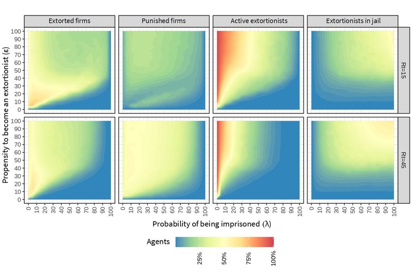
The percentage of active extortionists (not in jail) is inversely related to \(\lambda\), i. e., if the value of \(\lambda\) increases, the percentage of active extortionists decreases and vice versa. This process is catalyzed by \(R_t\), which accelerates the efficiency of the police. Accordingly, the percentage of extortionists in jail is directly related with \(\epsilon\) and \(\lambda\), since higher percentages of incarcerated are obtained when increasing both the propensity to become an extortionist and the probability of being imprisoned. Again, increasing \(R_t\) accelerates the effect of \(\lambda\), as it can be seen by comparing the size of the yellow regions.
Parameter-robustness analysis
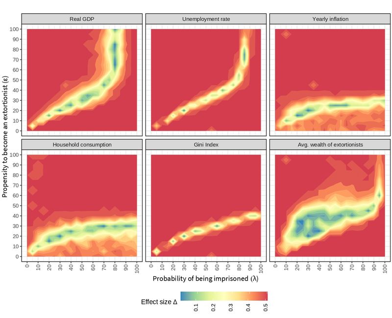
Figure 6 displays the \(\Delta\) effect size for the variables of interest as computed by the Test-A of Vargha & Delaney (2000). Based on the thresholds defined for this test (see Table 4), reddish regions denote large differences with respect to the default setting (see Table 2), while bluish regions denote small to medium differences. A variable is considered to be robust if it shows small to medium differences in the surroundings of the default parameter values, i.e., when \(\lambda=30\) and \(\epsilon=20\).
The following four variables are robust to changes in \(\lambda\) (keeping \(\epsilon\) constant at its default value): Production, inflation, consumption and average wealth of the extortionists. The average wealth of extortionists is also robust to changes in \(\epsilon\) (keeping \(\lambda\) constant at its default value). Though, unemployment and the Gini index are sensitive to parametrization and their behavior may not be considered as an emergent property of the model.
Color patterns in these heat maps show variables that have a similar behavior when changing the parameters \(\lambda\) and \(\epsilon\). For instance, see the shape for the real GDP and the unemployment rate or that of inflation and household consumption. The nature of these relationships is further explored along the paper.
The plots also reveal alternative combinations of the parameters that behave similarly to the default values. For instance, when \(\lambda=80\) and \(\epsilon=70\), the real GDP shows a small difference with the one obtained from the default values. Note that there is no combination of parameters globally equivalent to the default values, i.e., producing bluish regions in the same coordinates for all variables. Therefore, a single public policy can not influence all these economic variables simultaneously, e.g., if there is a desire to maintain production at a similar level to that emerging from the default setting, a new chosen policy will likely vary inflation, household consumption and the distribution of wealth.
This robustness analysis gives a first insight into the patterns and emerging properties of the BAMERS model. In the following section, the origin of such patterns is analyzed in more detail, as well as the interrelationships between the variables under study.
Macroeconomic effect of extortion
This section evaluates the effect of extortion on the economic variables of interest to this work. We analyze each of the variables in isolation as well as the interrelation of some variables that explain the economy as a whole. Heat maps are used to represent the values obtained when changing the parameters, where bluish regions refer to low values while reddish regions denote high values of the simulated variable.
Production, unemployment and inflation
Figure 7 shows the effect of extortion on the three main macroeconomic variables: production, unemployment and inflation. Regarding the real GDP, a contraction is observed when increasing the propensity to become an extortionist, which is accentuated in the presence of low probabilities of being imprisoned. As expected, the probability of being imprisoned works as a stabilizer of the economy by suppressing the detrimental effect of crime propensity on society.
The rejection threshold \(R_t\) acts as a parameter that increases the number of denounces by firms and it is a catalyst that accelerates the effect of \(\lambda\). For higher values of \(\epsilon\), getting the real GDP back to a value that is nearer to the base economy with no crime (\(\epsilon = 0\)) needs increasing the probability of imprisoning criminals but, while \(R_t=15\) requires an efficiency of \(\lambda \geq 80\), \(R_t=45\) asks for a lower efficiency of \(\lambda \geq 40\).
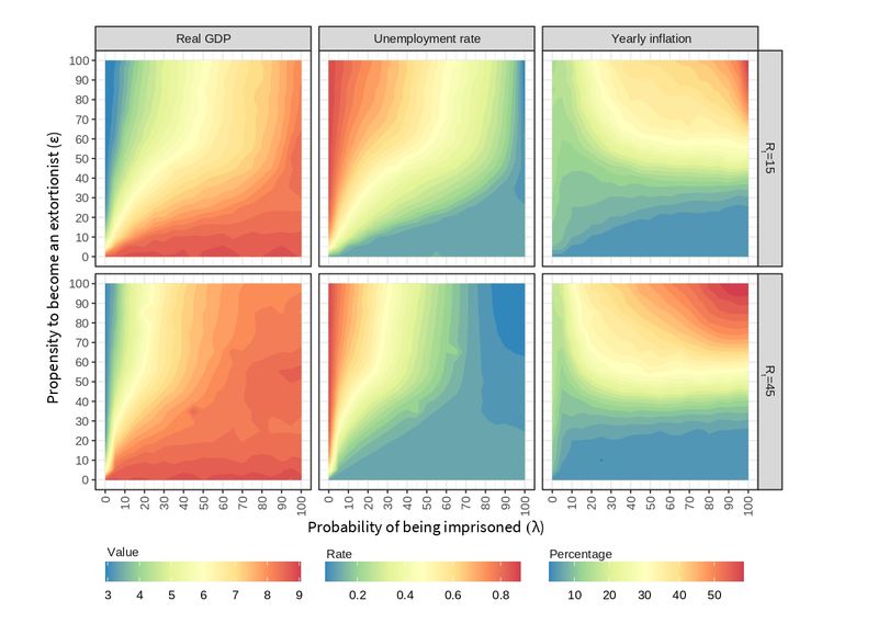
A clear effect of the propensity to become an extortionist on the value of production is also observed. The real GDP is sensitive to extortion, decreasing when \(\epsilon\) goes from from 0 to 10 and remarkably going down when \(\epsilon\) reaches 20. Increasing \(\epsilon\) any further has only a marginal decreasing effect on production because the system gets saturated of extortionists with a limited number of firms to extort.
Unemployment rate increases when raising the propensity to become an extortionist and it decreases when the probability of being imprisoned is higher. Note how this is the reverse situation of that observed for the real GDP, which suggests that unemployment and production follow the Okun’s Law (Furceri et al. 2019) in our simulation. The so-called Okun’s law suggests a bivariate negative relationship between unemployment and production. By relying on the BAM model that maintains the productivity constant, the BAMERS model thus provides a policy tool to assess unemployment cost on aggregate supply.
The rejection threshold \(R_t\), makes the effect of \(\lambda\) more elastic. When \(R_t = 45\), more efficient labor allocations emerge in a rather unrealistic region where the propensity to become an extortionist is greater than 30 and the probability of being imprisoned is also high. This is due to the fact that a high percentage of extortionists is in jail for that combination of \(\epsilon\) and \(\lambda\) parameters, what decreases the number of agents that can be unemployed (see also Figure 5).
Inflation follows a different pattern when compared to the effect of \(\epsilon\), \(\lambda\) and \(R_t\) on production and unemployment in Figure 7. Inflation is in fact related to household consumption, measured as a proportion of goods produced in the economy, as it can be observed from the similar pattern shown in Figure 8.
The macroeconomic theory of inflation (Bronfenbrenner & Holzman 1963; Johnson 1963) establishes that one of its possible determinants in the short term is related to the contraction of aggregate supply or the increase in aggregate demand (or a combination of both). In our case, given that the region with the highest inflation occurs with a high propensity to become an extortionist combined with a high probability of being imprisoned, the trigger appears to be a small amount of labor in the formal sector, which reduces the aggregate supply with a constant aggregate demand.
Consumption
Two different indicators have been used to analyze consumption. First, household consumption measures aggregate consumption as a proportion of the goods produced in the economy. As it was previously discussed, aggregate consumption follows a similar pattern to that observed in yearly inflation (see Figure 8, left). It can be noticed that the highest consumption ratio is generated when there is both a high propensity to become an extortionist and a high probability of being imprisoned. In this situation, the scarcity of productive labor, which generates goods, leads to a contraction of the aggregate supply. Therefore, although the economy seems to be more efficient, an inflationary process is induced. The BAMERS model exhibits a negative effect of extortion on the supply side, which is in line with the negative effects of crime found by Astarita et al. (2018).
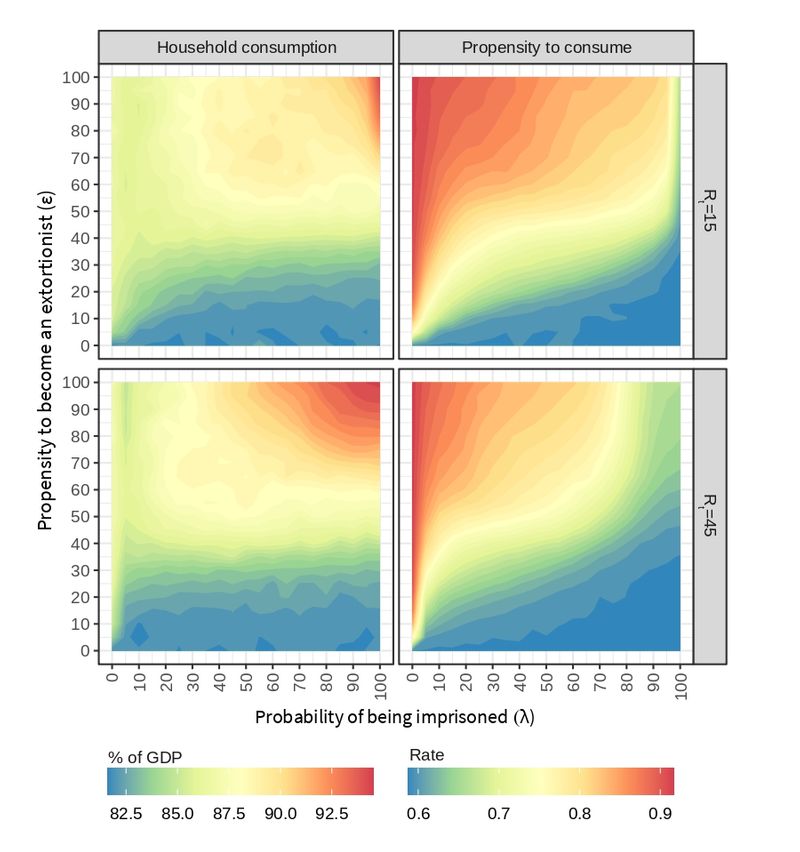
Second, the propensity to consume measures individual consumption as the proportion of wealth workers require to meet their needs. This variable behaves the same as the unemployment rate (see Figure 8, right). In the presence of crime (\(\epsilon > 0\)), \(\lambda\) manages to recover the economy with the help of \(R_t\). Note that the purchasing power of people is reduced in conditions of high unemployment rate, i.e., low probability of being imprisoned and presence of crime in society. In these situations, although some workers migrate to the criminal sector, they find a limited number of companies to extort and their success is not at all guaranteed. Saturating the economy with extortionists and keeping \(\lambda = 0\) leads to the highest propensity to consume, that is, a situation in which workers need to allocate the largest proportion of their wealth to survive.
Wealth distribution
In what follows, we analyze the Gini index as a commonly used measure of wealth distribution (Lerman & Yitzhaki 1984) and we also look at the skewness of wealth distributions as reported in related work by Delli Gatti et al. (2011) and Troitzsch (2014).
Figure 9 shows the inequality in the distribution of wealth among workers, measured as the Gini index resulting from the simulations for each combination of the parameters \(\lambda\), \(\epsilon\) and \(R_t\). Again, a pattern emerges in which \(\lambda\) mitigates the negative effect of crime. Inequality is harder to fight for higher values of \(\epsilon\), but the effect of \(\lambda\) can be accelerated when \(R_t\) is higher. Situations in which a high proportion of wealth is concentrated in a small proportion of workers are accentuated when the probability of being imprisoned is low.
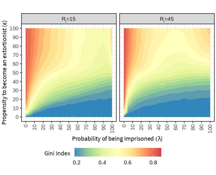
Figure 10 shows the bias observed in the distribution of wealth for regular workers, firms, and extortionists. Skewness remains positive for most of the combinations of \(\lambda\) and \(\epsilon\), thus confirming the stylized fact found in the literature about the positive bias of wealth distributions.
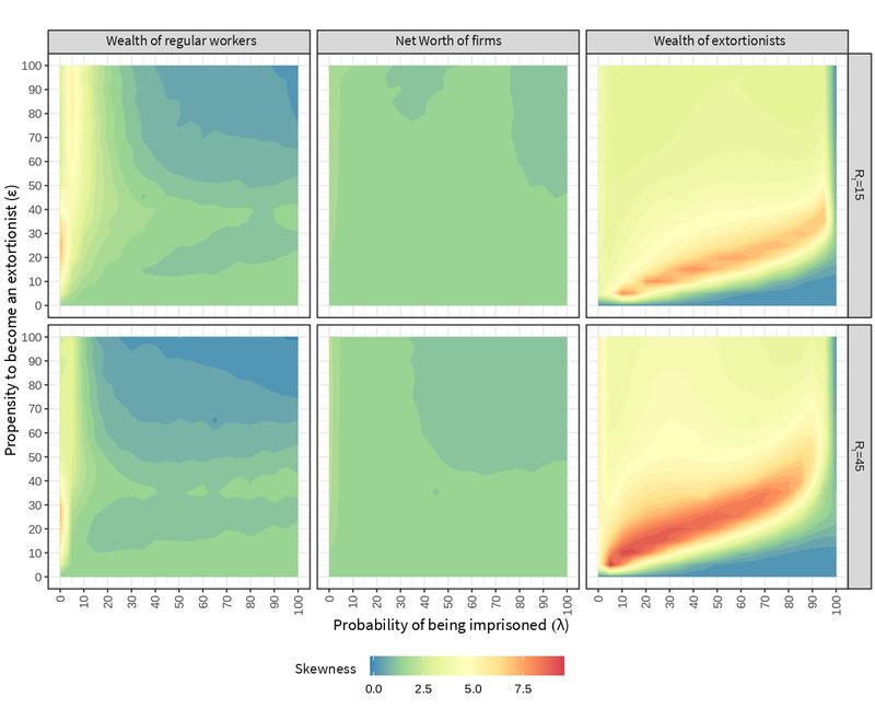
For regular workers, an increase in bias is only observed for moderate extortion levels (\(10 \leq \epsilon \leq 30\)) and an unrealistic low probability of being imprisoned (\(\lambda \approx 0\)). \(\lambda\) maintains its regulatory function with \(R_t\) as a catalyst of such stabilization. There is a region showing less inequality for regular workers, where skewness tends to zero. In this region, high values of \(\epsilon\) reduce the number of regular workers while high values of \(\lambda\) raise the number of imprisoned extortionists. As a result, the confiscated money from prisoners makes their wealth to more balanced once they are released.
Skewness in the distribution of the net worth of firms does not show any significant change when varying the parameters. We recall that punished firms receive an equal proportion of the victim support fund raised from the wealth of the extortionists in jail.
The higher skewness obtained for the wealth of extortionists tells about the risk or volatility of this type of criminal activity. As Troitzsch (2014) pointed out, few extortionists become successful, the main determinant for low success being the "prosecution propensity". In our model, this is accentuated in the scenario with a greater tendency to denounce. The reddish regions show a phase where the probability of being imprisoned is enough to imprison a high proportion of extortionists in the system. This area is wider when the tendency to denounce is greater, since more attempts are generated to imprison extortionists.
The positive biases found in all wealth distributions comply with the stylized fact reported in the literature, regardless the change in its magnitude when varying the model parameters \(\epsilon\) and \(\lambda\).
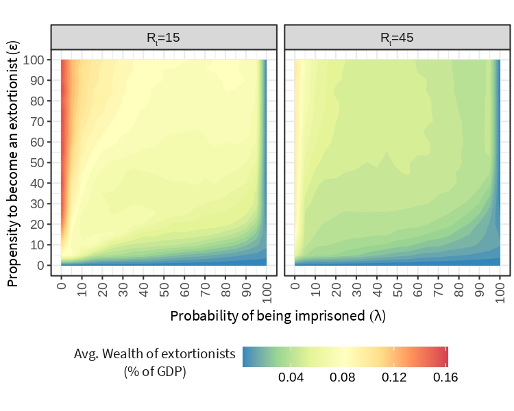
Figure 11 shows the average wealth of extortionists as a proportion of the GDP. Increasing \(\epsilon\) makes the average wealth of extortionists grow. Raising the rejection threshold makes extortionists less wealthy, even when \(\lambda\) is zero and there are no extortionists in jail. Still, \(\lambda\) has a stronger effect in this scenario, where the higher number of denounces helps the police to decrease the average wealth of extortionists.
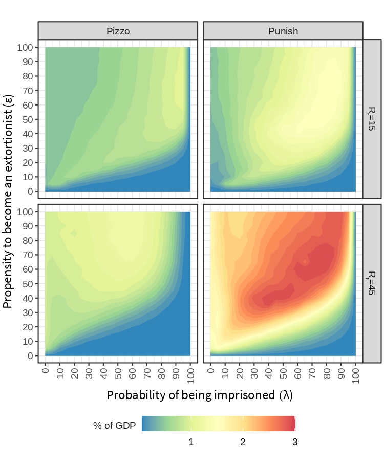
The amount of money that flows into crime is increased through punishment, i.e., extortionists collectively obtain a greater amount of income through punishment than from pizzo (see Figure 12). \(R_t\) is a catalyst that further increases crime income, since it raises the number of denounces and, consequently, it also increases the level of punishment. \(\lambda\) continues to have a stabilizing effect on the economy. Though, the highest revenue is not collected for low probabilities of being imprisoned but it is obtained in specific regions where both the propensity to become an extortionist and the probability of being imprisoned are higher. In this sense, the frontal fight against crime seems to be beneficial for a selected group of extortionists. Competition and risk is higher in these scenarios but so it is the reward they can obtain.
A counter intuitive trade-off emerges from the previous results. If the objective is to reduce criminal profits, the efficiency of the police should better be either limited or extremely high (the latter being rather unrealistic). On the other hand, if the objective is to improve macroeconomic indicators (regardless of the profit of criminal organizations), the police must be as efficient as possible.
Comparing distributions of macroeconomic signals
So far we have analyzed the response of the macroeconomic variables to changes in the model parameters. We now use the non-parametric Cucconi Test to check whether the distribution of the signals is different also in terms of their dispersion, i.e., the location-scale problem (Marozzi 2009; Murakami 2016).
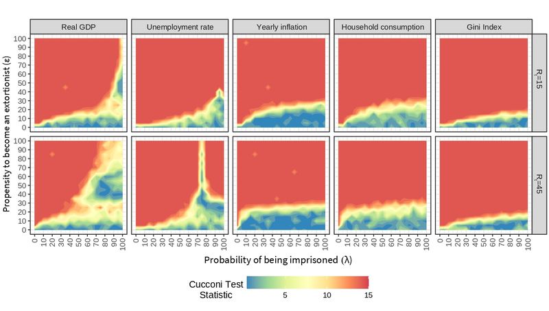
The sample distribution generated with the baseline macroeconomic model without extortion (\(\epsilon = 0\)) is compared against all combinations of extortion (\(\epsilon \geq 0\)) and efficiency of the police (\(\lambda \geq 0\)). The value of the test statistic is expected to be zero if the macroeconomic signals have no differences in both treatments; but if distributions differ in the mean and/or variance, the value of the statistic will be greater than zero. The greater the difference, the greater the value of the statistic. In the experimentation carried out, the value of the Cucconi Test statistic varies between 0 and 15 (see Figure 13).
A global view of these plots suggests an effect of extortion on economic variables. Bluish regions represent scenarios in which the behavior of the variables is statistically similar to that observed without crime. In turn, yellow regions can be seen as boundaries where small changes of parameters can lead to notable changes. Reddish regions represent scenarios in which the behavior of the variables is statistically different to that observed without crime. These phase transitions emerge from the BAMERS model as a function of \(\epsilon\), \(\lambda\), and \(R_t\) for all the variables of interest, excepting unemployment at \(R_t=45\), that exhibits three phases, the third one showing unrealistic low levels of unemployment.
Policies can be designed that are oriented towards the desired directions. However, it must be observed that not all variables exhibit this effect exactly in the same way, e.g., the real GDP shows a broader margin of recovery when compared to the Gini index, which can not be recovered when \(\epsilon \geq 20\). The same goes for inflation and consumption, although with a higher span of control. Designing a general policy that brings the economy under extortion closer to a ideal state (such as that observed in the absence of crime) means trying to keep all variables in the blue region, which is not always possible. Therefore, the decision maker needs to be aware of trade-offs and, sometimes, put a lower priority on some of the indicators to mitigate the effect of crime on other variables.
Conclusion
Beyond being a kind of tax that increases the cost of firms, extortion is also a source of fear that spreads throughout the economic system, decreasing investment and growth (Elsenbroich et al. 2016). Our simulation shows that even low levels of propensity towards becoming an extortionist are enough to notice considerable negative effects on macroeconomic indicators such as the real GDP and the unemployment rate. Such an impact corroborates the observations of Astarita et al. (2018) on Italian data that show a decrease in economic activity when facing criminal activities.
The BAMERS model can help to analyze what could be done to reduce the effect of extortion on the economy. Our simulation results suggest that preventing extortion may be more effective than combating it, i.e., there is no value of the probability of being imprisoned that achieves the levels of the baseline economy of the overall macro variables observed when extortion propensity is more than 15%. Even though, both policies should be evaluated in terms of monetary cost to determine their feasibility.
The results also suggest that macroeconomic variables have a less elastic reaction to changes in the probability of being captured than to changes in the propensity to become an extortionist, with the exception of the real GDP, where high \(\lambda\) values can still reproduce values close to those observed in the setting without crime.
One way of preventing extortion and discourage the proliferation of criminals is to make this activity less profitable. According to the output of our simulation, the average wealth of criminals is strongly related to the rejection threshold applied by firms when deciding whether to accept paying the pizzo. By increasing the number of denounces, firms can help decrease the average wealth of criminals, although this also depends on the probability of being captured as previously suggested by Troitzsch (2014). An effective and reputed justice system could be a way to raise this rejection threshold.
The propensity to become an extortionist (\(\epsilon\)), the probability of being imprisoned (\(\lambda\)) and the rejection threshold (\(R_t\)) are orthogonal by design in the BAMERS model, i.e., we can explore any combination of these parameters exhaustively but independently. To overcome this limitation, the inclusion of learning agents is proposed as future work, e.g., studying how \(\epsilon\) self-regulates as a result of extortionists learning in response to the effectiveness of the criminal justice system expressed by \(\lambda\).
The lack of credibility in the justice system has been pointed out as an empirical cause for the spread of extortion (La Spina et al. 2014). Improving the reputation of the entire justice system, e.g., by increasing the efficiency of criminal conviction, would prevent extortion to the extent that the population becomes aware of such efficiency. However, issues such as trust, credibility, or reputation were out of the scope of this research and remain as future work. The results of the GLODERS project about the normative patterns that promote and maintain extortion racket systems will be very useful for this purpose.
Other causes for the proliferation of extortion rackets systems may also be considered. For instance, in Latin America, extortion is strongly linked to a context of exclusion and deprivation, which involves poverty, indigents and bad income distribution (Anzola et al. 2016). BAMERS opt for exploring how existing agents in the BAM model might become extortionists as a result of their context. Abrahamsen (1949) provided a plausible, although not general, explanation of how this happens. Observe that this simplification defines the way extortionists appear in the system together with the propensity to become extortionist (\(\epsilon\)). Since this parameter is explored exhaustively during experimentation, we found it suffices for studying the effect of different levels of extortion in the simulated economy.
BAMERS can be used to verify if, the fact that extortionists always come from the poorest quartile of the population, bias the results in some sense by, for instance, changing the code for selecting them from a different part of the population and comparing then the obtained results with the old ones. But of course, such modification is no longer supported by Abrahamsen’s work. In this sense, BAMERS is a useful tool for testing alternative explanations of the way extortion emerges. As future work, we aim to evaluate the effect of public policies for the attention to the economic deprivation of workers in reducing social discontent and, therefore, decreasing the propensity to become extortionists.
From a macroeconomic point of view, the BAMERS model allowed us to understand the behavior of the fundamental variables describing an economy under a specific type of crime such as extortion. By altering parameters such as the probability of capturing extortionists as well as the threshold of rejection to pay the pizzo, we were able to establish conditions that generate desirable and undesirable scenarios, which will shed light on the design of macroeconomic policies that are beneficial for society as a whole.
Notes
- BAM model: https://www.comses.net/codebases/9dacc220-8d7f-4038-b618-92bb9b1333f0/.
- GLODERS project: https://cordis.europa.eu/project/id/315874.
- BAMERS model: https://www.comses.net/codebases/e03074bc-714e-47b3-b01d-c0b6b2e61380/.
Appendix: ODD protocol of the BAM model
Overview
Purpose: Exploring the use of an agent-based approach for the study of macroeconomic signals. Particularly, we are interested in applying the BAM model to study the effect of agent behavior on such signals.
Entities, state variables and scales:
- Agents: Firms, workers and banks.
- Environment: A 2D grid is used as visual aid for debugging, but it is meaningless with respect to the model.
- State variables: The attributes that characterize each agent are shown in Table 4.
- Scales: Time is represented in discrete periods, each one represents a month.
| Agent | Variable | Type | Agent | Variable | Type |
|---|---|---|---|---|---|
| Firm | production-Y | Int | Worker | employed? | Bool |
| desired-production-Yd | Int | my-potential-firms | AgSet | ||
| expected-demand-De | Int | my-firm | Ag | ||
| desired-labor-force-Ld | Int | contract | Int | ||
| my-employees | AgSet | income | Float | ||
| current-num-employees-L0 | Int | savings | Float | ||
| num-of-vacancies-offered-V | Int | wealth | Float | ||
| minimum-wage-W-hat | Float | prop-to-consume-c | Float | ||
| wage-offered-Wb | Float | my-stores | AgSet | ||
| net-worth-A | Float | my-large-store | Ag | ||
| total-payroll-W | Float | Bank | total-amount-of-credit-C | Float | |
| loan-B | Float | patrimonial-base-E | Float | ||
| my-potential-banks | AgSet | operational-interest-rate | Float | ||
| my-bank | AgSet | interest-rate-r | Float | ||
| inventory-S | Float | my-borrowing-firms | AgSet | ||
| individual-price-P | Float | bankrupt? | Bool | ||
| revenue-R | Float | ||||
| retained-profits-pi | Float |
Process overview and scheduling. The main loop of the simulation is as follows:
Firms calculate production based on expected demand.
A decentralized labor market opens. Unemployed workers look for a job.
A decentralized credit market opens. Banks will lend money to firms.
Firms produce.
A market for goods opens and workers buy.
Firms pay loans and dividends.
Firms and banks survive or go bankrupt.
Firms and banks that go bankrupt are replaced.
Design concepts
Basic Principles: The model follows fundamental principles of neoclassical economics (Woodford 2009), since it gives great importance to money in economic processes and also because the strategy for determining prices is given, considering both supply and demand.
Emergence: The model generates adaptive behavior of the individual agents, without the imposition of a global equation that governs their actions. Macroeconomic signals are also emergent properties of the system.
Adaptation: Based on the evidence of survey data (See Delli Gatti et al. (2011), p. 55), the BAM model assumes that the firms can adapt either the price or the amount of goods supplied, i.e., only one of them, at each step. Adaptation depends on the situation of the firm (supply-demand balance in the previous period) and the market (difference between the own and the market price).
Objectives: Agents do not have an explicit objective value but, implicitly, they try to improve a utility or attribute, e.g., workers always opt for the best known wage and price.
Learning: None for the moment, however, see the future work section for possible uses of learning in this model.
Prediction: Firms predict the quantity of goods to be produced based on the excess of supply-demand in the previous period and the difference between their own price and the average market price.
Sensing. Different for each kind of agent:
Firms perceive their own quantity of goods produced, individual price, labor force, net worth, profits and offered wages; as well as the average market price and the interest rate of randomly chosen banks.
Workers perceive the size of firms visited in the previous period, the prices published by firms in the actual period and the wages offered by firms.
Banks perceive the net worth of potential borrowers to calculate interest rates.
Interaction. Interactions among agents are determined by the markets:
In the labor market, firms post their vacancies at a certain offered wage. Then, unemployed workers contact a given number of randomly chosen firms to get a job, starting from the one that offers the highest wage. Firms have to pay the wage bill in order to start production. A worker whose contract has just expired applies first to his/her last employer.
Firms can access to a decentralized credit market if their net worth is in short supply for the wage bill. Borrowing firms contact a given number of randomly chosen banks and apply for a loan starting from the one charging the lowest interest rate. Banks sort applications in descending order according to the financial soundness of firms, and satisfy them until all credit supply has been exhausted. The contractual interest rate is calculated applying a mark-up on an exogenous determined baseline interest rate. After the credit market is closed, if financial resources are not enough to pay for the wage bill of the population of workers, some workers remain unemployed or are fired.
In the goods market, firms post their offer price, and workers contact a given number of randomly chosen firms to purchase goods, starting from the one which posts the lowest price.
Stochasticity: Random shocks are introduced in the setting of wages (\(\xi\)) and contractual interest rates (\(\phi\)). Also in the strategies to set prices (\(\eta\)) and quantities to produce (\(\rho\)).
Collectives: Markets configure collectives of agents, they include labor, goods, and credit markets. In addition, firms and workers are categorized as rich and poor.
Observation: Gross Domestic Product (GDP), unemployment, inflation and interest rate are observed along the simulation. Distribution of firm sizes, workers’ wealth and GDP growth rate are computed by the end of the simulation.
Details
Initialization: Table 6 shows the initialization parameters of the model, which are mainly taken from Delli Gatti et al. (2011) or experimentally determined when not provided in the previous text.
| Parameter | Value | Parameter | Value | ||
|---|---|---|---|---|---|
| \(I\) | Number of consumers | 500 | \(H_\eta\) | Maximum growth rate of prices | 0.1 |
| \(J\) | Number of producers | 100 | \(H_\rho\) | Maximum growth rate of quantities | 0.1 |
| \(K\) | Number of banks | 10 | \(H_\phi\) | Maximum amount of bank’s costs | 0.1 |
| \(T\) | Number of steps | 1000 | \(Z\) | Number of trials in the goods market | 2 |
| \(C_P\) | Propensity to consume (poor) | 1 | \(M\) | Number of trials in the labor market | 4 |
| \(C_R\) | Propensity to consume (rich) | 0.5 | \(H\) | Number of trials in the credit market | 2 |
| \(\sigma_P\) | R&D investment of poorest firms | 0 | \(\hat{w}\) | Minimum wage (by law) | 1 |
| \(\sigma_R\) | R&D investment of richest firms | 0.1 | \(P_t\) | Aggregate price | 1.5 |
| \(h_\xi\) | Maximum growth rate of wages | 0.05 | \(\delta\) | Fixed fraction to share dividends | 0.15 |
Input data: None, although data from real economies might be used for validation.
Submodels: Agent behavior is defined as follows:
- Production \(Y\) and technological productivity \(\alpha\): \(Y_ {it} = \alpha_{it} L_{it}\), s.t., \(\alpha_{it}> 0\), where \(L\) is the labor factor of firm \(i\) at time \(t\).
- Desired production level \(Y_ {it} ^ d\) is equal to the expected demand \(D_ {it} ^ d\).
- Desired labor force (employees) \(L_ {it} ^ d = Y_ {it} ^ d / \alpha_ {it}\).
- Number of vacancies offered by firms \(V_ {it} = max (L_ {it} ^ d - L_ {it} ^ 0, 0)\).
- Current number of employees \(L_ {it} ^ 0\) is the sum of employees with a valid contract.
- If there are no vacancies (\(V_ {it} = 0\)), wage offered is \(w_ {it} ^ b = max (\hat {w_t}, w_ {it-1})\), where \(\hat {w_t}\) is the minimum wage determined by law.
- If \(V_{it} >0\), wage offered is \(w_ {it} ^ b = max (\hat {w_t}, w_ {it-1} (1+ \xi_ {it}))\), where \(\xi_ {it}\) is a random term evenly distributed between \((0, h_{\xi})\).
- At the beginning of each period, a firm has a net worth \(A_ {it}\). If total payroll to be paid \(W_ {it} > A_ {it}\), firm asks for loan \(B_ {it} = max (W_ {it} - A_ {it}, 0 )\).
- Firms look for a limited number banks in the credit market \(H<K\) since applying for a loan is considered an expensive task.
- In each period the \(k\)-th bank can distribute a total amount of credit \(C_k\) equivalent to a multiple of its patrimonial base \(C_ {kt} = E_ {kt} / v\), where \(0 < v <1\) can be interpreted as the capital requirement coefficient. Therefore, the \(v\) reciprocal represents the maximum allowed leverage by the bank.
- Bank offers credit \(C_ {k}\), with an interest rate \(r_ {it} ^ k\) and contract for 1 period.
- If \(A_ {it + 1}> 0\) the payment scheme is \(B_ {it} (1 + r_ {it} ^ k)\).
- If \(A_ {it + 1} \leq 0\), bank retrieves \(R_ {it + 1}\).
- Contractual interest rate offered by the bank \(k\) to the firm \(i\) is determined as a margin on a rate policy established by Central Bank \(\bar {r}\), s.t., \(R_ {it} ^ k = \bar {r} (1+ \phi_ {kt} \mu (\ell_ {it}))\).
- Margin is a function linked to each bank as possible variations in its operating costs and captured by the uniform random variable \(\phi_ {kt}\) in the interval \((0, h_\phi)\).
- Margin is also a function of the borrower’s financial fragility, captured by the term \(\mu (\ell_ {it})\), \(\mu' > 0\). Where \(\ell_ {it} = B_ {it} / A_ {it}\) is the leverage of borrower.
- Demand for credit is divisible, i.e., if a single bank is not able to satisfy the requested credit, it can request in the remaining \(H-1\) randomly selected banks.
- Each firm has a stock of unsold goods \(S_ {it}\), where excess supply \(S_ {it}> 0\) or demand \(S_ {it} = 0\) is reflected.
- Deviation of the individual price from the average market price during the previous period is represented as: \(P_ {it-1} - P_ {t-1}\)
- If deviation is positive \(P_ {it-1}> P_ {t-1}\), firm recognizes that its price is high compared to its competitors, and is induced to decrease the price or quantity to prevent a migration massive in favor of its rivals; and vice versa.
- In case of adjusting price downward, this is bounded below \(P_ {it} ^l\) to not be less than your average costs:
\[P_ {it} ^ l = ( W_ {it} + \sum\limits_k r_ {kit} B_ {kit} ) / Y_ {it}\] Aggregate price \(P_t\) is common knowledge, while stock \(S_ {it}\) and individual price \(P_ {it}\) are private.
Only the price or quantity to be produced can be modified. In the case of price, we have the following rule:
where: \(\eta_ {it}\) is a randomized term uniformly distributed in the range \((0, h_ \eta)\) and \(P_ {it} ^ l\) is the minimum price at which firm \(i\) can solve its minimal costs at time \(t\). [model:price-shocks]\[\begin{aligned} P_{it}^s= \begin{cases} \text{max}[P_{it}^l, P_{it-1}(1+\eta_{it})] & \text{if $S_{it-1}=0$ and $P_{it-1}<P$ }\\ \text{max}[P_{it}^l, P_{it-1}(1-\eta_{it})] & \text{if $S_{it-1}>0$ and $P_{it-1}\geq P$} \end{cases} \end{aligned}\] In the case of quantities, these are adjusted according to:
where \(\rho_ {it}\) is a random term uniform distributed and bounded between \((0, h_ \rho)\).\[\begin{aligned} D_{it}^e= \begin{cases} Y_{it-1}(1+\rho_{it}) & \text{if $S_{it-1}=0$ and $P_{it-1}\geq P$} \\ Y_{it-1}(1-\rho_{it}) & \text{if $S_{it-1}>0$ and $P_{it-1}< P$} \end{cases} \end{aligned}\] - Total income of workers is the sum of the payroll paid to the workers in \(t\) and the dividends distributed to the shareholders in \(t-1\).
- Wealth is defined as the sum of wage plus the sum of all savings \(SA\) of the past.
- Marginal propensity to consume \(c\) is a decreasing function of the worker’s total wealth (the higher the wealth the lower the proportion spent on consumption):
where \(SA_t\) is the average savings. \(SA_ {jt}\) is the real saving of the \(j\) -th consumer.\[c_ {jt} = 1 / (1+ \left [\text {tanh} \left ( SA_ {jt} / {SAt} \right) \right] ^ \beta)\] - The revenue \(R_ {it}\) of a firm after the goods market closes is \(R_{it} = P_ {it} Y_ {it}\).
- At the end of \(t\) period, each firm computes benefits \(\pi_ {it-1}\).
- If the benefits are positive, shareholders receive dividends \(Div_ {it-1} = \delta \pi_ {it-1}\).
- Residual, after discounting dividends, is added to net worth from previous period \(A_{it-1}\). Therefore, net worth of a profitable firm in \(t\) is:
\[A_{it} = A_{it-1}+\pi_{it-1} -Div_{it-1} \equiv A_{it-1}+ (1-\delta)\pi_{it-1}\] - If firm \(i\) accumulates a net worth \(A_ {it} <0\), it goes bankrupt.
- Firms that go bankrupt are replaced with another one of size smaller than the average of incumbent firms. Non-incumbent firms’ size is above and below 5%.
- Bank’s capital:
\[E_{kt}=E_{kt-1} + \sum \limits_ {i \in \Theta} r_ {kit-1} B_ {kit-1} -BD_{kt-1}\] - \(\Theta\) is the bank’s loan portfolio, \(BD_{kt-1}\), i.e, firms that go bankrupt.
- Bankrupted banks are replaced with a copy of one of the surviving ones.
References
ABRAHAMSEN, D. (1949). Family tension, basic cause of criminal behavior. Journal of Criminal Law and Criminology (1931-1951), 40(3), 330–343. [doi:10.2307/1138546]
ALDEN, K., Read, M., Timmis, J., Andrews, P. S., Veiga-Fernandes, H., & Coles, M. (2013). Spartan: A comprehensive tool for understanding uncertainty in simulations of biological systems. PLoS Computational Biology, 9(2), 1–9. [doi:10.1371/journal.pcbi.1002916]
ALVES-FURTADO, B., & Eberhardt, I. D. R. (2016). A simple agent-based spatial model of the economy: Tools for policy. Journal of Artificial Societies and Social Simulation, 19(4), 12: https://www.jasss.org/19/4/12.html.
ANDRIGHETTO, G., Brandts, J., Conte, R., Sabater-Mir, J., Solaz, H., Székely, Á., & Villatoro, D. (2016). Counter-punishment, communication, and cooperation among partners. Frontiers in Behavioral Neuroscience, 10(53). [doi:10.3389/fnbeh.2016.00053]
ANDRIGHETTO, G., Giardini, F., Paolucci, M., Prisco, A., Renzi, D., & Azadi, S. (2016). Bell’ esempio! Esperienza partecipativa e studio sperimentale sull’ autonomia normativa dei bambini attraverso le multe morali. Sistemi Intelligenti, 28(1), 33–48.
ANZOLA, D., Neumann, M., Möhring, M., & Troitzsch, K. G. (2016). 'National mafia-type organisations: Local threat, global reach.' In C. Elsenbroich, D. ANZOLA, & N. Gilbert (Eds.), Social Dimensions of Organised Crime: Modelling the Dynamics of Extortion Rackets (pp. 9–23). Berlin: Springer International Publishing. [doi:10.1007/978-3-319-45169-5_2]
ASTARITA, C., Capuano, C., & Purificato, F. (2018). The macroeconomic impact of organised crime: A post-Keynesian analysis. Economic Modelling, 68, 514–528. [doi:10.1016/j.econmod.2017.08.029]
BRONFENBRENNER, M., & Holzman, F. D. (1963). Survey of inflation theory. The American Economic Review, 53(4), 593–661.
CHRISTIANO, L. J., Eichenbaum, M. S., & Trabandt, M. (2018). On DSGE Models. Journal of Economic Perspectives, 32(3), 113–140. [doi:10.1257/jep.32.3.113]
CUCCONI, O. (1968). Un nuovo test non parametrico per il confronto fra due gruppi di valori campionari. Giornale Degli Economisti E Annali Di Economia, 27(3-4), 225–248.
DAWID, H., & Delli Gatti, D. (2018). 'Agent-based macroeconomics.' In C. Hommes & B. LeBaron (Eds.), Handbook of Computational Economics (Vol. 4, pp. 63–156). Amsterdam, NL: Elsevier.
DE Grauwe, P. (2010). Top-Down versus Bottom-Up Macroeconomics. CESifo Economic Studies, 56(4), 465–497. [doi:10.1093/cesifo/ifq014]
DELLI Gatti, D., & Desiderio, S. (2015). Monetary policy experiments in an agent-based model with financial frictions. Journal of Economic Interaction and Coordination, 10(2), 265–286. [doi:10.1007/s11403-014-0123-7]
DELLI Gatti, D., Desiderio, S., Gaffeo, E., Cirillo, P., & Gallegati, M. (2011). 'Macroeconomics from the bottom-up.' In New Economic Windows (Vol. 11). Berlin: Springer. [doi:10.1007/978-88-470-1971-3]
ELSENBROICH, C., Anzola, D., & Nigel, G. (2016). Social Dimensions of Organised Crime: Modelling the Dynamics of Extortion Rackets. Berlin Heidelberg: Springer.
ELSENBROICH, C., & Badham, J. (2016). The extortion relationship: A computational analysis. Journal of Artificial Societies and Social Simulation, 19(4), 8: https://www.jasss.org/19/4/8.html. [doi:10.18564/jasss.3223]
EVANS, P. (2000). US stylized facts and their implications for growth theory. School of Economics; Finance, University of Hong Kong.
FAGIOLO, G., & Roventini, A. (2017). Macroeconomic policy in DSGE and agent-based models redux: New developments and challenges ahead. Journal of Artificial Societies and Social Simulation 20 (1) 1: https://www.jasss.org/20/1/1.html. [doi:10.18564/jasss.3280]
FURCERI, D., Jalles, J. T., & Loungani, P. (2019). On the determinants of the Okun’s Law: New evidence from time-varying estimates. Comparative Economic Studies, 62, 661–700. [doi:10.1057/s41294-019-00111-1]
GAMBETTA, D. (1996). The Sicilian Mafia: The Business of Private Protection. Cambridge, MA: Harvard University Press.
GRIMM, V., Berger, U., Bastiansen, F., Eliassen, S., Ginot, V., Giske, J., Goss-Custard, J., Grand, T., Heinz, S. K., Huse, G., Huth, A., Jepsen, J. U., Jørgensen, C., Mooij, W. M., Müller, B., Pe’er, G., Piou, C., Railsback, S. F., Robbins, A. M., … DeAngelis, D. L. (2006). A standard protocol for describing individual-based and agent-based models. Ecological Modelling, 198(1-2), 115–126. [doi:10.1016/j.ecolmodel.2006.04.023]
GRIMM, V., Berger, U., DeAngelis, D. L., Polhill, J. G., Giske, J., & Railsback, S. F. (2010). The ODD protocol: A review and first update. Ecological Modelling, 221(23), 2760–2768. [doi:10.1016/j.ecolmodel.2010.08.019]
GUALDI, S., Tarzia, M., Zamponi, F., & Bouchaud, J.-P. (2015). Tipping points in macroeconomic agent-based models. Journal of Economic Dynamics and Control, 50, 29–61. [doi:10.1016/j.jedc.2014.08.003]
GUTIERREZ-GARCIA, J. O., Orozco-Aguirre, H., & Landassuri-Moreno, V. (2013). Agent-based simulation of crime. 2013 12th Mexican International Conference on Artificial Intelligence. [doi:10.1109/micai.2013.9]
HARRIS, R. (1992). Testing for unit roots using the augmented Dickey-Fuller test : Some issues relating to the size, power and the lag structure of the test. Economics Letters, 38, 381–386. [doi:10.1016/0165-1765(92)90022-q]
HELTON, J. C. (2008). 'Uncertainty and sensitivity analysis for models of complex systems.' In F. Graziani (Ed.), Computational Methods in Transport: Verification and Validation (pp. 207–228). Berlin Heidelberg: Springer Berlin Heidelberg. [doi:10.1007/978-3-540-77362-7_9]
JOANES, D. N. & Gill, C. A. (1998). Comparing measures of sample skewness and kurtosis. Journal of the Royal Statistical Society. Series D (The Statistician), 47(1), 183–189. [doi:10.1111/1467-9884.00122]
JOHNSON, H. G. (1963). A survey of theories of inflation. Indian Economic Review, 6(3), 29–69.
KLIMEK, P., Poledna, S., Farmer, D. J., & Thurner, S. (2015). To bail-out or to bail-in? Answers from an agent-based model. Journal of Economic Dynamics and Control, 50, 144–154. [doi:10.1016/j.jedc.2014.08.020]
KONRAD, K. I., & Skaperdas, S. (1998). Extortion. Economica, 65(260), 461–477. [doi:10.1111/1468-0335.00141]
KYDLAND, F. E., & Prescott, E. C. (1982). Time to build and aggregate fluctuations. Econometrica, 50(6), 1345–1370. [doi:10.2307/1913386]
LA Spina, A., Frazzica, G., Scaglione, A., & Punzo, V. (2014). How Mafia works: An analysis of the extortion racket system. ECPR General Conference.
LEPAGE, Y. (1971). A combination of Wilcoxon’s and Ansari-Bradley’s statistics. Biometrika, 58(1), 213–217. [doi:10.1093/biomet/58.1.213]
LERMAN, R. I., & Yitzhaki, S. (1984). A note on the calculation and interpretation of the Gini index. Economics Letters, 15(3-4), 363–368. [doi:10.1016/0165-1765(84)90126-5]
LOTZMANN, U., Möhring, M., & Troitzsch, K. G. (2013). Simulating the emergence of norms in different scenarios. Artificial Intelligence and Law, 21(1), 109–138. [doi:10.1007/s10506-012-9130-y]
MACAL, C. M., & North, M. J. (2010). Tutorial on agent-based modelling and simulation. Journal of Simulation, 4(3), 151–162. [doi:10.1057/jos.2010.3]
MAROZZI, M. (2009). Some notes on the location-scale Cucconi test. Journal of Nonparametric Statistics, 21(5), 629–647. [doi:10.1080/10485250902952435]
MAROZZI, M. (2014). The multisample Cucconi test. Statistical Methods & Applications, 23(2), 209–227. [doi:10.1007/s10260-014-0255-x]
MORALES, V. P., Mar Vélez Salas, D. del, Rodrı́guez, F. J. R., & Salas, M. V. (2015). Evolución de la extorsión en méxico: Un análisis estadı́stico regional (2012-2013). Revista Mexicana de Opinión Pública, 18, 112–135.
MURAKAMI, H. (2016). All-pairs multiple comparisons based on the Cucconi test. AStA Advances in Statistical Analysis, 100(3), 355–368. [doi:10.1007/s10182-016-0268-x]
NARDIN, L. G., Andrighetto, G., Conte, R., Székely, Á., Anzola, D., Elsenbroich, C., Lotzmann, U., Neumann, M., Punzo, V., & Troitzsch, K. G. (2016). Simulating protection rackets: A case study of the Sicilian Mafia. Autonomous Agents and Multi-Agent Systems, 30(6), 1117–1147. [doi:10.1007/s10458-016-9330-z]
NARDIN, L. G., Székely, Á., & Andrighetto, G. (2017). GLODERS-S: A simulator for agent-based models of criminal organisations. Trends in Organized Crime, 20(1), 85–99. [doi:10.1007/s12117-016-9287-y]
PALLEY, T. (1998). Walras’ Law and Keynesian macroeconomics. Australian Economic Papers, 37(3), 330–340. [doi:10.1111/1467-8454.00023]
PARUNAK, H. V. D., Savit, R., & Riolo, R. L. (1998). 'Agent-based modeling vs. equation-based modeling: A case study and users’ guide.' In J. S. Sichman, R. Conte, & N. Gilbert (Eds.), First International Workshop, MABS’98 (pp. 10–25). Berlin Heidelberg: Springer-Verlag.
PLATAS-LÓPEZ, A., Guerra-Hernández, A., Cruz-Ramı́rez, N., Quiroz-Castellanos, M., Grimaldo, F., Paolucci, M., & Cecconi, F. (2020). 'Towards an agent-based model for the analysis of macroeconomic signals.' In O. Castillo, P. Melin, & J. Kacprzyk (Eds.), Intuitionistic and Type-2 Fuzzy Logic Enhancements in Neural and Optimization Algorithms: Theory and Applications (pp. 551–565). Berlin Heidelberg: Springer International Publishing.
PLATAS-LÓPEZ, A., Guerra-Hernández, A., Grimaldo, F., Paolucci, M., & Cecconi, F. (2019). Micro-foundations of macroeconomic dynamics: The agent-based BAM model. In J. Sabater-Mir, V. Torra, I. Aguiló, & M. González-Hidalgo (Eds.), Artificial intelligence research and development. Proceedings of the 22nd international conference of the catalan association for artificial intelligence. IOS Press.
REALPE-GÓMEZ, J., Vilone, D., Andrighetto, G., Nardin, L. G., & Montoya, J. A. (2018). Learning dynamics and norm psychology supports human cooperation in a large-scale Prisoner’s Dilemma on networks. Games, 9(4).
STIGLITZ, J. E. (2017). Where modern macroeconomics went wrong. Working Paper. Available at: http://www.nber.org/papers/w23795. [doi:10.3386/w23795]
TROITZSCH, K. G. (2014). Distribution effects of extortion racket systems. In F. Amblard, F. Miguel, A. Blanchet, & B. Gaudou (Eds.), Lecture Notes in Economics and Mathematical Systems (pp. 181–193). Berlin Heidelberg: Springer International Publishing. [doi:10.1007/978-3-319-09578-3_15]
TROITZSCH, K. G. (2017). Can agent-based simulation models replicate organised crime? Trends in Organized Crime, 20(1), 100–119. [doi:10.1007/s12117-016-9298-8]
VARGHA, A., & Delaney, H. (2000). A critique and improvement of the "CL" Common Language effect size statistics of McGraw and Wong. Journal of Educational and Behavioral Statistics, 25(2), 101–132. [doi:10.2307/1165329]
VENKATESH, S., & Chin, K.-L. (1997). Chinatown gangs: Extortion, enterprise, and ethnicity. Contemporary Sociology, 26, 747. [doi:10.2307/2654660]
VILLATORO, D., Andrighetto, G., Conte, R., & Sabater-Mir, J. (2015). Self-policing through norm internalization: A cognitive solution to the tragedy of the digital commons in social networks. Journal of Artificial Societies and Social Simulation, 18(2), 2: https://www.jasss.org/18/2/2.html. [doi:10.18564/jasss.2759]
WOODFORD, M. (2003). Interest and Prices: Foundations of a Theory of Monetary Policy. Princeton, NJ: Princeton University Press.
WOODFORD, M. (2009). Convergence in macroeconomics: Elements of the new synthesis. American Economic Journal: Macroeconomics, 1(1), 267–279. [doi:10.1257/mac.1.1.267]
WORLD Bank. (2019a). Inflation, consumer prices (annual %). Data retrieved from World Development Indicators: http://data.worldbank.org/indicator/FP.CPI.TOTL.ZG.
WORLD Bank. (2019b). Unemployment, total (% of total labor force) (national estimate). Data retrieved from World Development Indicator: http://data.worldbank.org/indicator/SL.UEM.TOTL.NE.ZS.