Agent-Based Model for Urban Administration: A Case Study of Bridge Construction and its Traffic Dispersion Effect

Introduction

As modern cities are expected to provide various functions to residents, the components associated with infrastructure have exponentially increased, and their interactions and structures have also become more complex. Recent advances in information and communication technologies (ICT), such as big data and artificial intelligence, have radically accelerated such trends. However, urban administrations, which should constructively respond to such demands and actively investigate directions for future city development, still face complex issues. This is why data-driven administration supported by ICT techniques is seen as a promising approach for handling these problems (Broomfield & Reutter 2021).

To better understand data-driven administration, research on urban traffic analysis deserves consideration for the following reasons: urban traffic requires infrastructure, and efficient planning and utilization of infrastructure facilitate various socio-economic activities, so it is closely related to urban administration. In this sense, urban traffic has been researched and the current research positively incorporates ICT, such as intelligent traffic systems (ITS) and new types of vehicles (e.g., personal mobility and autonomous vehicles; Chen et al. 2020). As urban traffic considers more components, simulation has been researched and then applied to the traffic analysis.

Traffic simulation is an abstraction of urban transportation systems. Hence, urban administrators can understand and analyze their current status through simulation results, which eventually help develop associated policies. In particular, the current issues in modern transportation and mobility systems, such as autonomous driving (i.e., self-driving vehicles), personal transportation (i.e., micromobility vehicles for transporting individuals at low speeds), and carbon neutrality (i.e., reducing carbon emissions from vehicles), have increased the need for simulation-based urban traffic analysis (Lu et al. 2020; Patella et al. 2019). The main advantage of traffic simulation is that it enables to evaluate future systems and policies which are not implemented yet (Arsham & Kahn 1990). For example, it can provide urban administrators with an awareness of where the future urban traffic systems should aim to cover, but realizing them is still complicated. In such cases, traffic simulation can be utilized as a sandbox to evaluate political considerations.

We propose a traffic simulation model and present a policy evaluation using the model. Specifically, our proposed model is an agent-based model in which agents representing city residents live their day using urban transportation, and their movements are determined by multiple decision processes derived from real data of the city residents. The proposed model estimates an urban traffic flow by aggregating individual movements, so it can be used to support urban traffic management including detecting traffic hot spots and mitigating traffic overheads. We note that while related works have often targeted simple or virtual cities, our proposed model describes a real city, Sejong, South Korea, and its population and traffic environments including road network and public transportation. Also, we utilized associated real data, such as individual characteristics (e.g., age, gender, occupation, living place) and time-use data from daily life, not only to model daily population movements, but to validate and calibrate our model.

Our case study illustrates an example of policy evaluations using the proposed traffic simulation model. As the developed model abstracts Sejong City, the case study dealt with its traffic considerations and formulated them into feasible policy candidates. We then conducted virtual experiments reflecting these policy candidates and quantitatively evaluated them using our simulation results. The main objectives of our case study were to answer the following research questions:

RQ1. Identify the traffic dispersion effect of new bridge construction according to location. In the case study, we considered the new bridge construction scenarios for Sejong. Among several predetermined location candidates for new bridge construction, we identified the best candidate to solve the traffic jams experienced on existing bridges. By simulating the proposed model, we checked the traffic volume changes of existing bridges and the traffic demands of new bridges for each construction scenario. RQ2. Profile the traffic demands of new bridge construction according to location. We also analyzed the destinations of the traffic passing through the new bridges. We classified the new bridge traffic into subgroups by destination and specified preferred new bridge construction scenarios for each subgroup.

While the results support to identify the best option, the city administrators may doubt its credibility in practice. As such, simulation-based policy evaluation should make an effort to secure the result reliability. We made additional efforts to validate the developed model with the associated real data and to analyze the results of the virtual experiments in detail: the former was achieved by adapting real data during model validation and calibration; the latter was conducted by tracking the reasons behind evaluation results through analysis of individual movements logged during simulation execution. We noted that these efforts would help urban administrators not only to improve evaluation results’ credibility, but to gain a chance to understand multifaceted political factors and their complex relations in future city.

Related Works

This section presents a survey of the previous research related to the proposed work. We separated works into model development (including modeling theory and method) and model application (i.e., policy evaluation in urban administration) research.

Related works on traffic simulation models

Traffic simulation models are generally categorized into three types with respect to the modeling focus on the traffic system: macroscopic, microscopic, and mesoscopic model. Macroscopic model mainly focuses on capturing traffic dynamics, such as aggregated behavior about traffic flows and congestion behaviors, so it often abstracts details on traffic processes and conditions (Lighthill & Whitham 1955). On the contrary, microscopic model describes the interactions among individuals in the traffic systems, such as vehicles and pedestrians, so it can provide more feasible parameters which are more aligned with the real world. Mesoscopic model stands between these two model types, which means that it blends the properties of macroscopic and microscopic models to discover more efficient results.

A macroscopic traffic model normally describes traffic flow from the view of aggregated behavior in a traffic system; so, for example, it often abstracts a great number of vehicles on a road as traffic density. It is a traditional way to analyze traffic systems, which mainly concentrates on traffic demand and capacity (Brilon 2000). Because traffic flow is similar to fluid dynamics, methods of developing macroscopic traffic models also come from the field of fluid dynamics, which is based on partial differential equations. Hence, macroscopic models are often developed as mathematical models representing the relationships among traffic system features, such as density, flow, and mean speed in the road network (Khan & Gulliver 2018). Since the pioneering work suggested by Lighthill & Whitham (1955), many works have been conducted: for example, Helbing et al. (2001) proposed a macroscopic traffic simulation model based on a gas-kinetic traffic equation. Their model allowed analysis of the influences of street and weather conditions, as well as freeway control measures on traffic flow. Boel & Mihaylova (2006) presented a compositional stochastic model for freeway traffic simulation for large-scale road networks. Thonhofer et al. (2018) developed a flexible macroscopic traffic model for large-scale urban traffic simulation.

Microscopic traffic model concentrates on vehicle-driver combinations (often just referred to as a vehicle) at an individual level. Individual information can be specified and recorded at all times during simulation (Elefteriadou 2014). Due to such individual features, agent-based modeling (ABM) has recently been applied to develop microscopic traffic models. ABM is a general method to build simulation models through the interactions among agents (or individuals) and environments in a system (Bae & Moon 2015; Russell & Norvig 2009). For example, Hidas (2002) suggested an agent-based traffic simulation model to evaluate road congestion and dynamic route guidance. Klügl & Bazzan (2004) presented a simulation method for route choice decisions of individual drivers and traffic forecasts utilizing drivers’ decisions. Kumar & Mitra (2006) analyzed virtual traffic situations in which traffic signals malfunctioned, which were realized by modeling individual vehicles and road conditions in India.

Mesoscopic traffic model was proposed to fill the gap between the macroscopic and the microscopic traffic models. Specifically, mesoscopic traffic models generally describe the traffic entities in detail, but their behavior and interactions at a lower level of detail (Burghout 2004). The mesoscopic models can have various forms, but one representative example is Taylor (2003) where grouped vehicles are moving on the road network, and the speed of a vehicle is calculated from the speed-density function of the road that the grouped vehicles move on. The approach of Taylor (2003) has influenced to lots of later works: for example, Sun et al. (2020) evaluated the potential impacts of various levels of high occupancy vehicle lane usages with commercial mesoscopic models and Mihăiţă et al. (2019) built an simulation model describes traffic environmental changes inside the neighborhood including air pollution, traffic flow or meteorological information. The proposed model is also such extension: with traffic individuals incorporating its moving behavior extracted from the real-data and elaborating on the speed-density function for its moving speed. Table 1 shows the comparison between the proposed model and the above traffic simulation models.

Table 1: Comparisons of the proposed model and the previous traffic simulation models

Model Type	Literature	Research Content
Macroscopic	Helbing et al. (2001)	developed a gas-kinetic traffic equation based traffic model for traffic flow analysis
	Boel & Mihaylova (2006)	developed a compositional stochastic model for freeway traffic simulation model
	Thonhofer et al. (2018)	developed a flexible traffic model for large-scale urban traffic simulation
Microscopic	Hidas (2002)	developed an agent-based traffic simulation model for evaluating road congestion and dynamic road guidance
	Klügl & Bazzan (2004)	developed a simulation model for route choice decisions of individual drivers and traffic forecasts
	Kumar & Mitra (2006)	developed a simulation model for analyzing virtual traffic situations where traffic signals malfunctioned in India
Mesoscopic	Taylor (2003)	developed a simulation model where grouped vehicles are moving on the road network with the speed calculated by a speed density function
	Sun et al. (2020)	evaluated the potential impacts of various levels of high occupancy vehicle lane usages with commercial mesoscopic traffic simulation tools
	Mihăiţă et al. (2019)	built an simulation model describes traffic environmental changes inside the neighborhood including air pollution, traffic flow or meteorological information
	Ours	proposed a simulation model with traffic individuals incorporating its moving behavior extracted from the real-data and elaborating on the speed-density function for its moving speed

Related works on simulation-based policy evaluation

Let us introduce another view of the proposed method: the application perspective. Although there are numerous ways to utilize simulation models in socioeconomics, one of the best known and most promising methods is to use virtual experiments as a tool for complex administrative decisions or policy evaluation. Gilbert et al. (2018) stated that computation models, including simulation models, can be utilized to initiate, develop, and evaluate policies due to the policy development cycle’s complexity and variability (see HM Treasury 2013). There have been a number of works about simulation-based policy evaluation in various domains, such as economics (Coester et al. 2018; Yun & Moon 2020), demographics (Kim et al. 2017; Singh et al. 2018), and public health (Bae et al. 2018; Barbrook-Johnson et al. 2017). This research trend has also appeared in urban administrative studies using traffic simulations: for example, Adelt et al. (2018) argued that traffic simulation could be applied to analyze the governance of complex sociotechnical systems, but their efforts ended up being a conceptual framework and a virtual small example. Ge & Polhill (2016), Fagiolo & Roventini (2017) and Yücel & van Daalen (2009) all presented examples of policy evaluation based on traffic simulations.

Before considering simulation-based policy evaluation, the validity of our simulation model should be verified. If a simulation model is not sufficiently valid, the simulation results and evaluation based on those results will be unreliable as well. For this reason, a number of simulation studies have mentioned the importance of model validation (Chu et al. 2003), but several works have provided the validity of traffic simulation models (Lengyel & Friedrich 2019; Ziemke et al. 2021). This rareness mainly results from two reasons: first, the studies were not dealing with real traffic systems, so there were no traffic data for comparison at the start; second, even if the author abstracted real datasets, the data were not readily prepared for various administrative reasons.

We propose an urban traffic simulation model that is technically categorized as a mesoscopic traffic model: traffic flow is estimated macroscopically, and individual movement is modeled microscopically. Also, we utilized our model to evaluate urban administrative policies related to population movement. Ratrout & Rahman (2009) suggested that a traffic simulation model incorporating traffic demands would be more effective for local administrations to implement. From this perspective, our paper is a realization of this suggestion. Moreover, to enhance the reliability of our policy evaluation results, we conducted model validation with real data. Specifically, our proposed model abstracted a real city in South Korea, Sejong, to effectively validate and calibrate based on observed traffic data. We also tracked the reasons for policy evaluation results that seemed counterintuitive through simulated microscopic factors. Although detailed information follows in the Case Study section, we would like to note that this is why the proposed model was developed at the mesoscopic level as another approach compared to the conventional mesoscopic traffic models (Lee et al. 2001).

Development of Sejong city model

With our model, we aimed to generate the daily behavior and movement patterns of a city’s population. We modeled real-scale city infrastructure and population. Table 2 summarizes our model by listing the model’s input data, output data, and parameters. By simulating the model, we obtained behavioral and location information of individuals for each simulated time increment. It is possible to analyze the demand for transportation resources, such as road capacity and public transportation, from the movement patterns we generated. Counterfactual experiments are also possible, such as changing road networks, populations’ demographic characteristics, or populations’ preferences.

Table 2: List of input data, output data, and model parameters

Type	Name	Implication	Value (Source)
Input	Residence data	Residence location data of the entire Sejong city population	Sejong City Hall (private)
	MDIS data	Survey data on Korean’s demographics and occupations	Statistics Korea (2015)
	Time-use data	Survey data on Korean’s time usage	Statistics Korea (2014)
	GIS data: Road	Sejong city road network information	Korea Transport DB (2019)
	Business license data	Sejong city business license registration data	Sejong Public Data (2019a)
	Bus route data	Sejong city bus routes	Sejong Public Data (2019b)
	Bus schedule data	Sejong city bus timetables	Sejong Public Data (2019b)
Output	Agent log	Agent behavior and location information by time	-
	Road log	Road traffic volume and traffic speed information by time	-
	Bus log	Bus passenger and location information by time	-
	Bus stop log	Bus stop usage information by time	-
Parameters	\(N\)	Number of population agents	300,000
	\(T\)	Simulation time (1 unit = 1 minute)	1,440 units
	\(\alpha\) (calibration target)	Selection probability penalty in workplace assignment	2.2357 (range: [0.1, 10])
	\(\beta\) (calibration target)	Selection probability penalty in random destination selection	5.631 (range: [0.1, 10])
	\(\gamma\) (calibration target)	Conversion rate between commute time and commute distance	2886.2 (range: [500, 5000])
	\(\delta_1\) (calibration target)	Sigmoid slope of the first phase in traffic speed estimation	3.5519 (range: [1.5, 6])
	\(\delta_2\) (calibration target)	Sigmoid slope of the second phase in traffic speed estimation	2.1608 (range: [2, 7])
	\(\delta_3\) (calibration target)	Concatenation point adjustment between the two phases in traffic estimation	2.0278 (range: [1, 4])
	\(\delta_4\) (calibration target)	Weight for exponential moving average in traffic speed estimation	0.9362 (range: [0, 1])
	\(\kappa\)	Selection probability increase rate in transportation selection	0.001

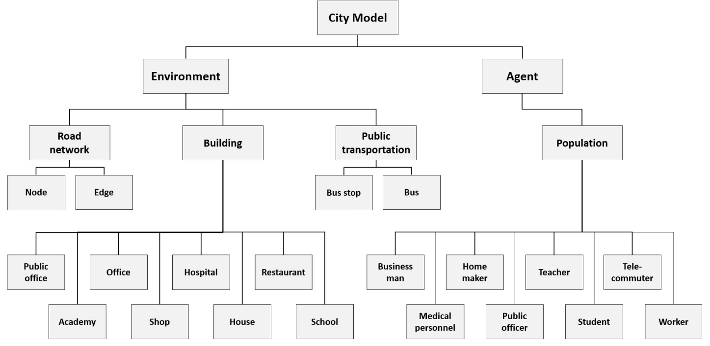
Our model consists of two main parts. One is the environment part, which represents urban infrastructure such as road networks, buildings, and public transportation. The other is the agent part, representing members of the population with heterogeneous occupations, such as businessman, homemaker, or teacher. Figure 1 summarizes the hierarchical structure of our model. In the following subsections, we describe the two modeling parts in detail.

Environment model

To model the city environment, we implemented a road network, buildings, and public transportation system. The environment influences population members’ behavior and movement. The road network affects the population’s movement routes. Buildings are needed for the population to perform their actions, so they serve as destinations for population movement. Last, the bus system provides an additional means of transportation for population movement besides private automobiles or walking. We implemented urban environments on the same scale as reality, using microlevel data from Sejong city. Table 3 summarizes the scale information of the model environments.

Table 3: Summary of model environment scale information

Environment	Type	Number	Description
Road network	Node	1,784	Based on Sejong road GIS data
	Edge	4,727	Based on Sejong road GIS data
Buildings	Residential	19,443	Based on Sejong building status data
	Nonresidential	13,127	Corresponds to each license in the business license data base
			(Public institutions and schools were manually added)
Bus system	Bus stops	3,208	Based on Sejong bus stop information
	Bus routes	116	Based on Sejong bus route information

Road network

To model Sejong’s road network, we used Sejong city road geographic information system (GIS) data provided by the Korean government (Korea Transport DB 2019). The road GIS data were in the form of a graph, with nodes indicating road intersections and endpoints and edges indicating roads. We referenced the graph structure and GIS data field to the structure and state variables of road network objects. Table 4 summarizes road network objects’ state variables.

Table 4: List of road network objects’ state variable

Object	State variable	Description	Value
Node	NODE_ID	Node identification number	GIS data constant
	NODE_TYPE	Node type information	GIS data constant
	Node_NAME	Node string name	GIS data constant
	TURN_P	Dummy variable for rotation restriction	GIS data constant
	GEOM	Node coordinates (Point)	-
Edge	LINK_ID	Edge identification number	GIS data constant
	F_NODE	Edge start node identification number	GIS data constant
	T_NODE	Edge end node identification number	GIS data constant
	ROAD_RANK	Road type information	GIS data constant
	ROAD_NAME	Road string name	GIS data constant
	MAX_SPD	Maximum traffic speed	GIS data constant
	LANES	Number of lanes	GIS data constant
	LENGTH	Road length	GIS data constant
	TRAFFIC_CNT	Traffic volume of the current simulation tick	Update via simulation
	TRAFFIC_SPD	Traffic speed of the current simulation tick	Update via simulation
	GEOM	Edge coordinates (Line)	-

Among the road network objects’ state variables, we updated the road traffic volume and speed at every simulation tick. Each road’s traffic volume was updated as the number of vehicles that passed over the road during the current simulation tick. Motivated by Delle Monache et al. (2021), who empirically demonstrated a three-phase relationship between road density and traffic speed, we estimated road traffic speeds using a function that concatenates two sigmoids with different slopes. Figure 2 shows this road traffic speed estimation function. \(\delta_{1}\), \(\delta_{2}\), and \(\delta_{3}\) are three model parameters that determine the shape of the traffic speed estimation function. First, \(\delta_{1}\) specifies the slope of the first-phase sigmoid function. Next, \(\delta_{2}\) specifies the slope of the second-phase sigmoid function. Last, \(\delta_{3}\) decides the concatenation point of the two sigmoid functions.

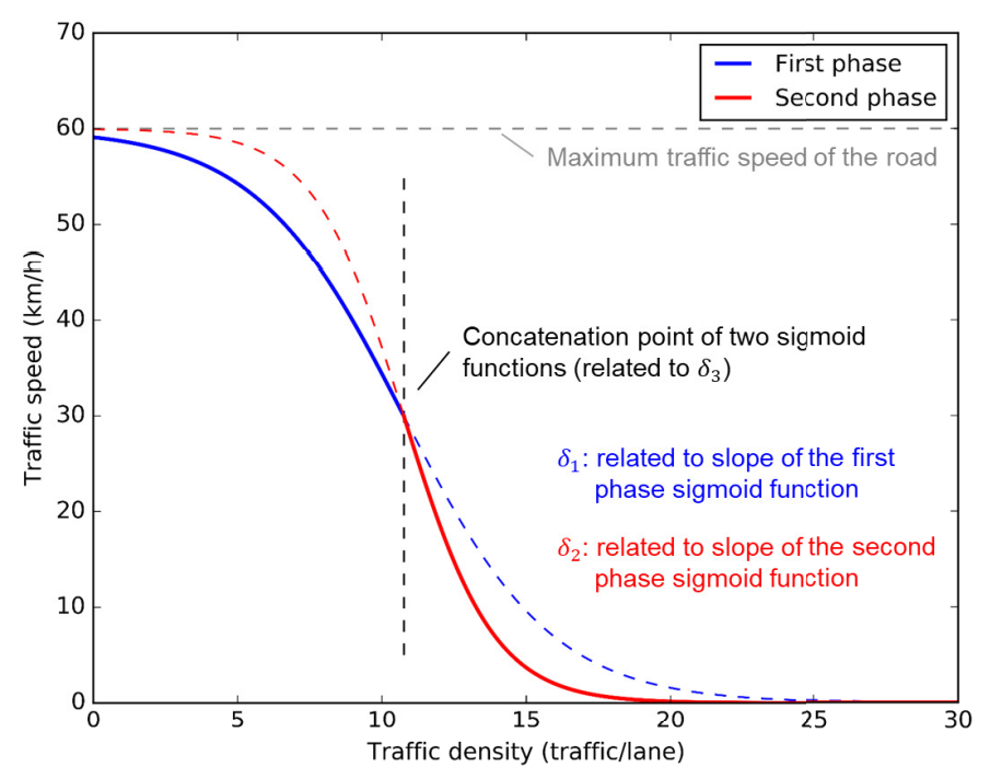
Also, we adopted an exponential moving average for the current road traffic speed estimation. Thus, the road traffic speed at the previous time affects the current road traffic speed. \(\delta_{4}\) is a weight parameter for the current value in the exponential moving average calculation. Taken together, we estimated the road traffic speed as follows.

\[\begin{split} V_{i,t} = \delta_{4} \times V_{i,t-1} + (1-\delta_{4}) \times \bigg[\frac{max\_spd_{i}}{1 + e^{\frac{ln(4)}{\delta_{1}}(D_{i,t-1} - \delta_{1} (\delta_{3} + 1))}} \times \textbf{1}_{(D_{i,t-1} \leq \delta_{1}(\delta_{3}+1))} \\ + \frac{max\_spd_{i}}{1 + e^{\frac{ln(4)}{\delta_{2}}(D_{i,t-1} - \delta_{1}(\delta_{3} + 1))}} \times \textbf{1}_{(D_{i,t-1} > \delta_{1}(\delta_{3}+1))} \bigg] \end{split}\]

\[(1)\]

Here, \(V_{i,t}\) is the traffic speed of road \(i\) at time \(t\); \(max\_spd_{i}\) is the maximum traffic speed of road \(i\) obtained from the road GIS data; \(\textbf{1}_{(condition)}\) is an indicator function that returns 1 when the conditions in parentheses are satisfied; \(D_{i,t}\) is the road density of road \(i\) at time \(t\), and the value is obtained from the road traffic volume divided by the road length and the number of road lanes; \(\delta_{1}\), \(\delta_{2}\), \(\delta_{3}\), and \(\delta_{4}\) are model parameters related to the traffic speed update process, and the calibrated values of each parameter are reported in Table 2.

Buildings and public transportation

For the building modeling, we generate several heterogeneous types of building objects. The building types are divided into residential buildings and nonresidential buildings. For the residential type building modeling, we employed Sejong city’s residence address data. This data is also used in the following agent initialization process, and detailed information about the data is summarized in Table 5. We create house type buildings at the data’s residence coordinates.

Next, to model nonresidential buildings, we use Sejong city business license data (Sejong Public Data 2019a). Sejong city licensing data has the following data fields: registered name, business type, address, and phone number. First, we converted the address information into coordinate form and then assigned each using the converted coordinates. The address’s floor information is not included in our modeling scope. Next, we assigned the building type according to the business type information. Population agents should be located in a building of the corresponding type to perform specific actions.

Last, we modeled bus routes as the model’s public transport. We implemented buses and bus stops using Sejong city bus stop data and route data (Sejong Public Data 2019b). Each bus departs from a departure station at the scheduled time. Then, it moves along the predetermined route and stops at the bus stops along the way. Finally, the bus arrives at its destination stop. Population agents are able to get on and off the bus only at the bus stops. Unlike personal vehicles, the bus’s speed is not limited by the road’s traffic speed at the time of passing. The bus has a constant moving speed, and it is not considered in the traffic volume calculation.

Agent model

Population agent modeling consists of two parts: the agent initialization part and the agent behavior modeling part. In the initialization step, we determined the population agents’ occupation type, then we assigned their residences and workplaces. In the behavior modeling step, we modeled decision-making rules regarding population agents’ behavior and movement.

Agent initialization

We use a combination of two microlevel data sets to initialize population agents. The first data set was Sejong city residence address data. It contained information on the age, gender, and detailed residence addresses of individuals living in Sejong city. The data cover the entire population of Sejong city in 2015. With this data, we performed a simulation with the actual population scale of Sejong city. However, this residence data did not include occupational information. Therefore, we could not create population agents with heterogeneous occupation types using only this residence data.

Table 5: List of data sets used in agent initialization process

Data	Properties	Value
Residence address data	Source	Sejong City Hall (anonymized, private)
	Sample period	2019
	Sample size	285,641 (full scale)
	Data field	Age, gender, and residence coordinates
MDIS data	Source	Statistics Korea
(microdata integrated service)	Sample period	2015
	Sample size	5,220 (Sejong citizens only)
	Data field	Age, gender, occupation type, commute time, etc.

To fill the residence data gap, we used an extra data set, the microdata integrated service (MDIS) data (Statistics Korea 2015). The MDIS data provides detailed demographic information from individual populations, including occupational information. However, it covers only about 2% of the total Korean population. Table 5 summarizes the two data sets we used in the population generation process.

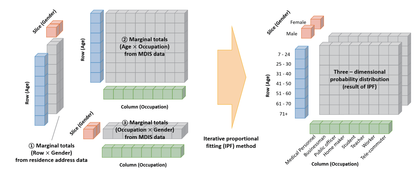
To generate population agents with heterogeneous occupation types, what we want to do is assign occupational information to the populations in the residence data. For this occupation assignment, we adopt an iterative proportional fitting method to generate a 3-dimensional probability distribution of age, gender, and occupation type. Figure 3 summarizes the probability distribution estimation task we performed. By applying the inferred distribution, we probabilistically assign the occupation types of the individuals in the residential data set. Also, we create population agents with heterogeneous occupation types.

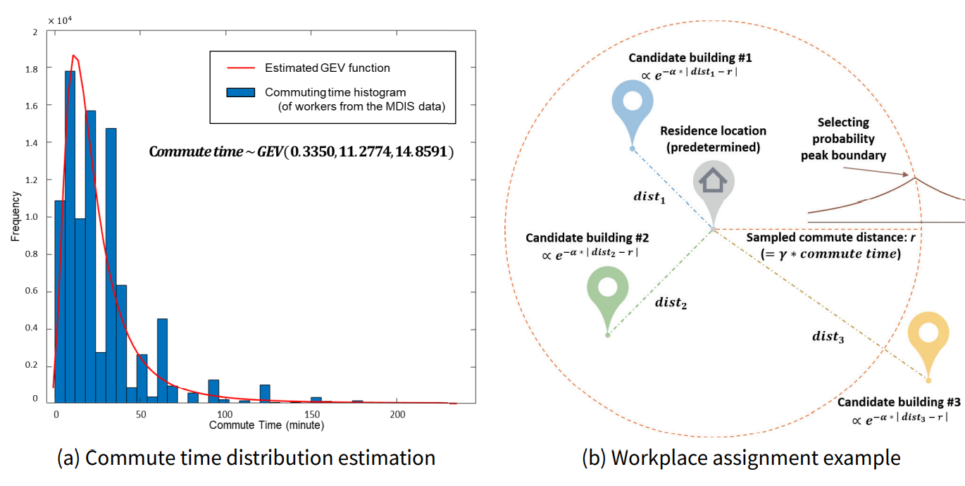
Then, we determine the agents’ residences using the residence coordinates data field of the residence data. We generate residential buildings at each coordinate and assign the generated buildings to agents as their residences. Next, for the workplace assignment, we first estimate the commute time of the MDIS data as a generalized extreme value (GEV) distribution, as shown in Figure 4a. Then, we randomly sample the commute time values of individual agents using the estimated GEV distribution. Lastly, we probabilistically assign each agent’s workplace using the predetermined residence location and the sampled commute time. Figure 4b is a graphical example of the workplace assignment process. In this process, we first convert the sampled commute time into commute distance. We assume a simple proportional relationship between the commute time and the commute distance and define the degree of this proportionality as the model parameter \(\gamma\). Therefore, \(\gamma\) determines the overall commute distances of individual agents. Next, we randomly select the workplace among the candidate buildings using the following formula, which penalizes the selection probability as the distance from the predetermined residence to the candidate building differs from the estimated commute distance. \(\alpha\) is a model parameter that adjusts the selection probability penalty according to this distance gap.

\[Prob(workplace = i) = \frac{e^{-\alpha \times \lvert dist_i - \gamma \times commute \; time \rvert}}{\Sigma_{i} e^{-\alpha \times \lvert dist_i - \gamma \times commute \; time \rvert}}\]

\[(2)\]

Here, \(dist_i\) is the Euclidean distance to building \(i\) from the agent’s residence location; \(commute \; time\) is the sampled commute time value from the estimated GEV distribution; \(\alpha\) and \(\gamma\) are model parameters related to working place assigning process, and the calibrated values of each parameter are reported in Table 2.

Agent behavior modeling

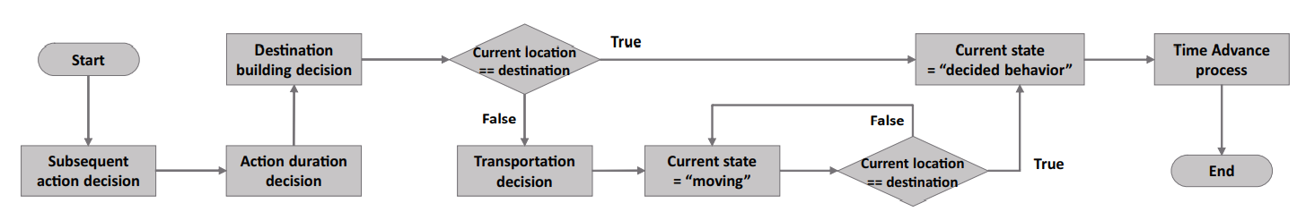
The population agent makes a series of decisions related to their actions and movements whenever they finish an action. In action-related decision-making, the population agent determines their subsequent action and the duration of this action. In movement-related decisions, the population agent selects a destination building for performing the predetermined action. Then, if the agent’s current location and the destination location are not the same, the agent decides on the transportation means and the route. Figure 5 depicts a flow chart modeling the overall agent behavior.

To model population agents’ behavioral patterns, we adopt time-use data surveying individuals’ behaviors every ten minutes during the day (Statistics Korea 2014). The time-use data were collected from 12,000 selected households, covering about 27,000 household members. The survey was conducted in three separate rounds in July, September, and November of 2014. Two days of time-use log and demographical information were surveyed for each respondent. As a result, this data’s sample size is 53,976. Table 6 summarizes the data field of the time-use data in detail.

Table 6: Data field summarization of time-use data

Data category	Data field name	Data type	Description
Demographics	AGE	double	Respondent’s age information
	GENDER	string	Respondent’s gender information
	EMPLOYMENT	string	Respondent’s employment status information
	OCCUPATION TYPE	string	Industry classification of respondent’s occupation
Time-use	DATE	string	Survey date
	STATE	list(string)	Respondent’s behavioral information during survey
			(The data is collected every ten minutes, 144 points per day)
	LOCATION	list(string)	Respondent’s location information during survey
			(The data is collected every ten minutes, 144 points per day)

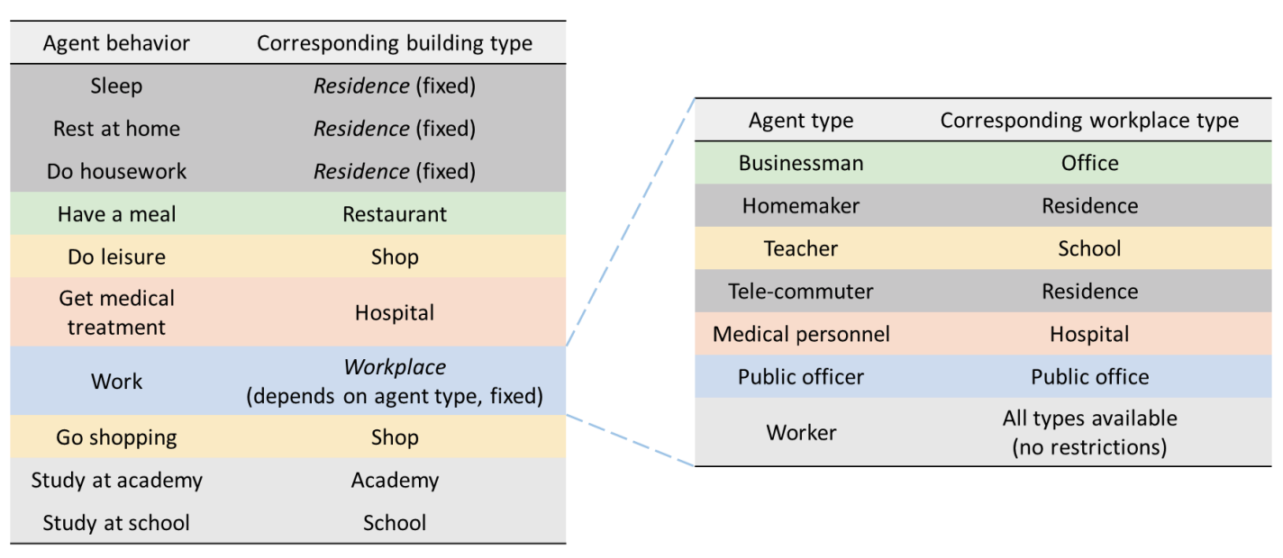
We modeled ten types of population agent behavior: sleep, rest at home, do housework, have a meal, do leisure, get medical treatment, work, go shopping, study at school, and study at academy. We classified the state information of the time-use data into these ten assumed action types. Similarly, we categorized the occupation information of the time-used data into the modeled occupation type. Occupational information enables us to generate heterogeneous behavioral patterns for each population agent type.

Using the time-use data, we first decide the agent’s subsequent behavior and then determine the duration of this behavior. Here, we consider the current time information at which the agents decide their ensuing action in addition to the agents’ occupation types. In reality, it is natural for the agents’ likely behaviors and their durations vary by time. For example, if you compare going shopping during working hours versus going shopping after work, the frequency and duration of shopping differ. Therefore, we calculate the probability of performing a specific action by agent occupation type and the time using the following formula. Through the estimated probabilities, we determine the population agent’s subsequent action.

\[Prob(action = s \; \lvert \; agent \; type = j \;\&\; time = t) = \frac{\Sigma_{i}\textbf{1}_{i}(j,s,t)}{\Sigma_{i}\textbf{1}_{i}(j,t)}\]

\[(3)\]

Here, \(\textbf{1}_{i}(conditions)\) is an indicator function that returns 1 when the population \(i\), surveyed individual of time-use data, satisfies the conditions in parentheses.

Next, we decided the subsequent action’s duration using the time-use data also consider the current time information. As common temporal information is considered in both behavior and duration determination processes, the association between behavior and its duration is implemented. From the data, we first collected instances among individuals with the same occupation type who performed the same action at the current time. Then, we measure how long the action continues after that point in the collected instances. From the counted durations, we estimate the mean and standard deviation of action duration by agent type and time using the following formulas. Here, we assume the distribution of action duration as a normal distribution.

\[\hat{\mu}_{j,s,t} = \frac{\Sigma_{i} [ duration_{i}(t) \times \textbf{1}_{i}(j,s,t) ]}{\Sigma_{i}\textbf{1}_{i}(j,s,t)}\]

\[(4)\]

\[\hat{\sigma}_{j,s,t} = \frac{\Sigma_{i} [ duration_{i}(t)^2 \times \textbf{1}_{i}(j,s,t) ]}{\Sigma_{i}\textbf{1}_{i}(j,s,t)} - \hat{\mu}_{j,s,t}^2\]

\[(5)\]

Here, \(\textbf{1}_{i}(conditions)\) is an indicator function that returns 1 when the population \(i\), surveyed individual of time-use data, satisfies the conditions in parentheses; \(duration_{i}(t)\) is the duration value of the action that population \(i\) is doing at time \(t\).

After the subsequent action is determined, the population agents select their destination buildings. Except for fixed-destination behaviors, the agents randomly select one of the buildings with a type corresponding to the action as a destination building. Figure 6 summarizes the agents’ behaviors and their corresponding building types. We modeled two intuitive assumptions about destination selection. One is that agents prefer nearby destinations. The other is that this preference for distance is stronger when the action’s duration is shorter. Under these assumptions, we calculate the probability that a building will be chosen as a destination using the following formula, which penalizes selection probability as the distance to the building increases. \(\beta\) is a model parameter that specifies this selection penalty according to the distance.

\[Prob(destination = i) = \frac{e^{-(\beta / ta) \times dist_i}}{\Sigma_{i} e^{-(\beta / ta) \times dist_i}}\]

\[(6)\]

Here, \(dist_i\) denotes the Euclidean distance to building \(i\) from the agent’s current location; \(ta\) is a behavior duration; \(\beta\) is a model parameter related to the destination selection process, and the parameter’s calibrated value is reported in Table 2.

In case the agent’s current location and destination location are different, the agents decide on a means of transportation to reach the destination. Agents with vehicles decide whether to travel by car or by public transport. The agents probabilistically select the traffic facility for each itinerary using the following formula, considering the parking location and the distance to the destination. In this formula, we make two intuitive assumptions. The first assumption is that agents will not use their car to move if the distance to pick up the car is farther than the destination. The second assumption is that the farther the destination is from the agent’s current location, the more likely the agent is to move by car. Here, \(\kappa\) is a model parameter related to the probability of moving by car according to the distance.

\[Prob(transportation = car) = max (1, \kappa * dist\_dest) \times \textbf{1} (dist\_car \leq dist\_dest)\]

\[(7)\]

Here, \(dist\_dest\) denotes the distance to the destination from the agent’s current location; \(dist\_car\) denotes the distance to the agent’s car from their current location; \(\kappa\) is a model parameter related to the transportaion selection, and the parameter’s assumed value is reported in Table 2.

Lastly, the population agents decide on their movement routes. We assume that population agents move only through the road network, except where there are no roads. If there is no road between the building and the nearest road node, the population agent moves between them in a straight line. On the road network, the population agent moves along the calculated shortest time path. For searching for the shortest time path, we adopt the Dijkstra algorithm and the A* algorithm. When calculating the shortest time path, the travel time value obtained by dividing the road length by the moving speed is used as the edge weight value. The moving speed value varies depending on the means of movement. Walking has a fixed moving speed regardless of road traffic. In the case of cars, however, their moving speed depends on the traffic speed of the road they are on. However, because we cannot predict the future road traffic speed at which the vehicle will pass, we use the most recent road traffic speed as the moving speed for the shortest time path search.

Case Study

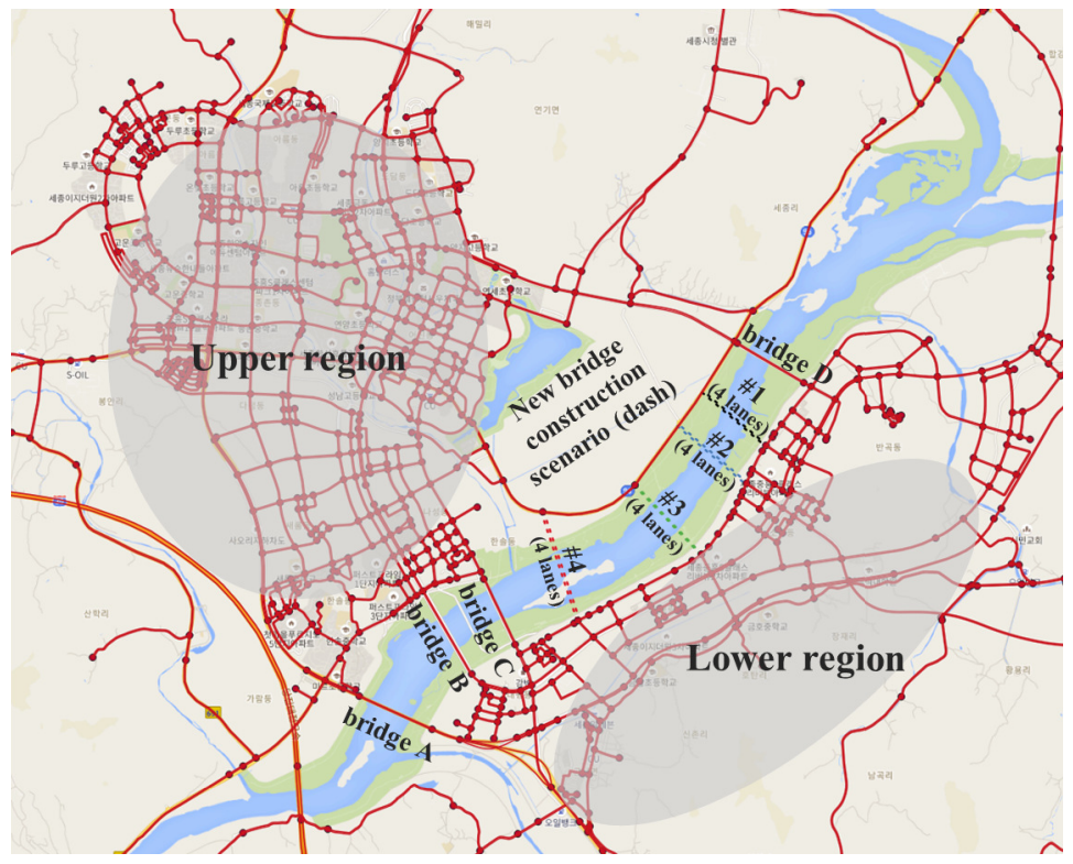
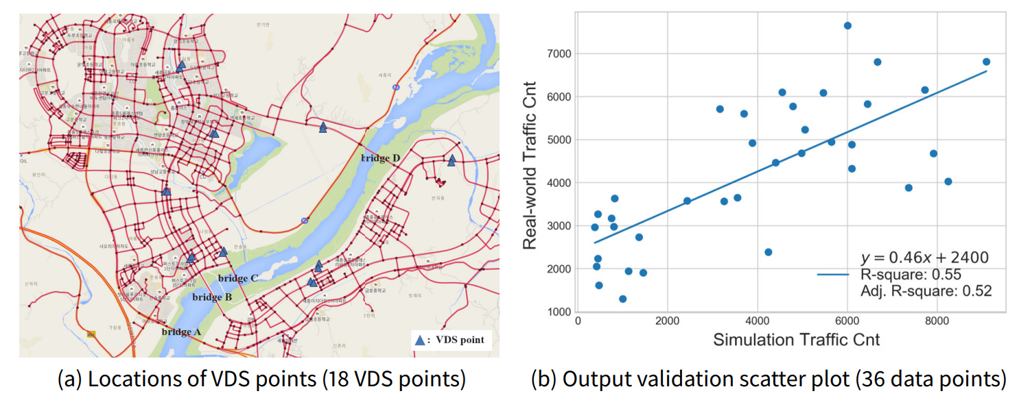
We conducted a policy experiment for new bridge construction using the Sejong city model. In Figure 7, there are four existing bridges (Bridge A, B, C, and D) between the river’s upper and lower regions. Population agents trying to move between the two areas must go through these bridges. The bridges cannot currently meet transport demand, resulting in traffic congestion. To address the existing bridges’ traffic congestion, we want to analyze the effect of traffic dispersion according to the new bridge construction. Additionally, we intend to provide policy implications for the optimal location for the new bridge construction through comparisons between the location candidates. We indicate the four predetermined location candidates of the new bridge construction using dashed lines (#1, #2, #3, and #4) in Figure 7.

Output validation

Before the policy experiment, we performed output validation to ensure the model’s validity. Output validation is a type of model validation that makes the simulation output and the corresponding real-world historical data similar (Manson 2003). In the output validation process, we compared the road traffic data collected from the real-world vehicle detection system (VDS) with the traffic of the corresponding road in the model. We selected a total of 36 VDS points around the new bridge construction candidate for output validation. Figure 9 a shows the VDS points’ locations for output validation on the map.

As a proxy for traffic discrepancy between simulation and reality, we evaluate how well the points, which have the VDS traffic volume and simulated traffic volume as their coordinate values, fit into an arbitrary linear model of the following form. We first estimate the linear regression model that best describes the points. Then, we calculate the R-squared statistic of the regression as a quantitative measure of this fitness.

\[\overline{y}_{i,t} = \beta_0 + \beta_1 \times \overline{x}_{i,t}\]

\[(8)\]

Here, \(\overline{y}_{i,t}\) is the average traffic volume during period \(t\) of the VDS point \(i\), and \(\overline{x}_{i,t}\) is the average traffic volume during period \(t\) of the corresponding road \(i\) in the model. For the time period, we divide days into day time (06:00–14:00) and evening time (14:00–22:00).

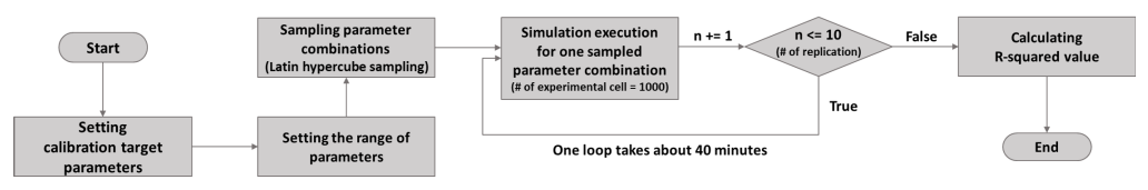
Figure 8 summarizes our entire output validation process. We first set the search space for the calibration target parameters. The lists of calibration target parameters and their range information are reported in Table 2. After that, we sample 1,000 parameter combinations in the defined parameter space using the Latin hypercube sampling method (McKay et al. 1979). We simulate ten replications for each parameter combination. Then, we calculate the R-squared value, which is the assumed proxy for the model validity, for each parameter combination. Lastly, we calibrated the model parameter values to the values of the combination with the largest R-squared value. The calibrated parameter values are summarized in Table 2. Figure 9b depicts the output validation results. In the scatter plot, each point represents a traffic volume pair of simulation output and real-world historical data for each VDS point and time. The R-squared value obtained from the best parameter combination is 0.55.

Our rationale for using the model selection metric, the R-squared statistic, as a model validity proxy is that our modeling scope covers a large area. Barde & van der Hoog (2017) asserted that a model selection metric such as Akaike information criterion (AIC) or Bayesian information criterion (BIC) may be better as a validation target in large-scale agent-based modeling. Also, some studies dealing with large urban areas adopted the R-squared discrepancies measure to check their models’ validities (Bieker et al. 2015; Gao et al. 2010).

The R-squared measure is a less intuitive discrepancy measure than the mean absolute percentage error (MAPE) or the mean squared error (MSE). The MAPE and the MSE measure discrepancy with stationary targets, whereas the R-squared measures discrepancy with the estimated linear models, which are moving targets.¹ However, when fitting a model using the MSE measure, we experience a tendency to calibrate by focusing on a few points with large residuals. When we fit the model using the R-squared measure, although there is a large discrepancy in the overall scale, we experience that the relationships between the points are more accurately reproduced. One of our modeling purposes is to cover a large area of the city, and we want to perform a relatively even verification over the entire area. The R-squared, which fits overall trends rather than focusing on a few points, is a more suitable measure for this modeling purpose.²

Policy experiment

In a policy experiment for new bridge construction, we experiment with four predetermined candidate locations (Scenarios #1, #2, #3, and #4 in Figure 7). We generate road GIS data with the new bridge for each construction scenario. We assume that the new bridge would have four lanes for every scenario, identically. The remaining input data and model parameters are the same as the baseline scenario. The baseline scenario refers to the current road GIS without new bridges. We simulated 20 iterations for each construction scenario, including a baseline scenario. We analyze the simulation results from the macroscopic and microscopic perspectives, respectively. First, as a macroscopic analysis, we check existing bridges’ and the new bridge’s traffic volume. From this result, we verify the new bridge’s traffic dispersion effect. Second, as a microscopic analysis, we performed destination profiling for the bridge passengers. The result of this profiling helps us achieve a better understanding of the new bridge’s demand.

Macroscopic result analysis

For the first part of the policy experiment, we summarize the experimental results related to RQ1 mentioned in the introduction section. To identify the traffic dispersion effect of the new bridge according to its location, we compare the traffic volume of existing bridges for each bridge construction scenario. The existing bridges’ traffic reduction amounts indicate the effectiveness of traffic dispersion according to the location of the new bridge. In other words, less traffic volume on the existing bridges implies a better new bridge location scenario.

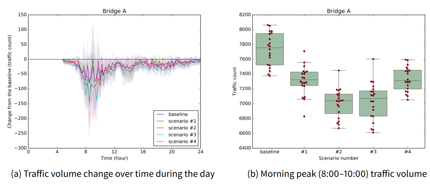
First, we check the traffic volume change of each existing bridge during the day. Figure 10a shows the changes in traffic volume of the existing bridge A over time compared to the baseline scenario for each bridge construction scenario. Because the figure denotes the change from the baseline, the blue line representing the baseline scenario becomes a horizontal line at zero. Next, we compare the bridge traffic during the morning peak (8:00–10:00), when the traffic is most congested. In Figure 10b, we compare bridge A’s morning peak traffic volume by the scenarios. Lastly, to check the significance between the scenarios, we conduct a statistical comparison between the morning peak traffic results. Table 7 statistically verifies whether bridge A’s morning peak traffic is significantly different among the construction scenarios. As a statistical analysis method, we conduct the Tukey honest significant difference (HSD) test (Tukey 1949). This test statistically checks whether the population’s means are significantly different from scenario to scenario. In the table, rejection of the null hypothesis implies that the two scenarios’ population means have a significant difference. Also, less traffic indicates the scenario with less traffic in the two compared scenarios.

Table 7: Tukey HSD test (FWER = 0.05, Bridge A)

Scenario (I)	Scenario (J)	Mean diff. (J-I)	Lower	Upper	p-value	Reject	Less traffic
baseline	#1	-420.25	-600.48	-236.02	0.001	True	#1
baseline	#2	-726.10	-910.33	-541.87	0.001	True	#2
baseline	#3	-704.9	-889.13	-520.67	0.001	True	#3
baseline	#4	-400.6	-584.83	-216.37	0.001	True	#4
#1	#2	-305.85	-490.08	-121.62	0.001	True	#2
#1	#3	-284.65	-468.88	-100.42	0.001	True	#3
#1	#4	19.65	-164.58	203.88	0.9	False	-
#2	#3	21.2	-163.03	205.43	0.9	False	-
#2	#4	325.5	141.27	509.73	0.001	True	#2
#3	#4	304.3	120.07	488.53	0.001	True	#4

We modeled ten types of population agent behavior: sleep, rest at home,

From the results of bridge A, the first identifiable implication is that the construction of a new bridge reduces the traffic volume of the existing bridge regardless of its location. In construction scenarios #1, #2, #3, and #4, the traffic volume of bridge A decreased compared with the baseline scenario. As a second implication obtained from the results, we check an inverted U-shape relationship between the inter-bridge distance and the traffic dispersion effect. As the new bridge location gets closer to the existing bridge, the new bridge has a greater traffic dispersion effect on the existing bridge. In scenarios #2 and #3, the traffic volume of bridge A is further reduced compared with in scenario #1. On the other hand, if the location of the new bridge is too close to the existing bridge, the new bridge’s traffic dispersion effect on the existing bridge is rather reduced. In comparison, between scenarios #3 and #4, scenario #3 has a greater traffic dispersion effect than scenario #4 does, even though the location of scenario #4 is closer to bridge A.

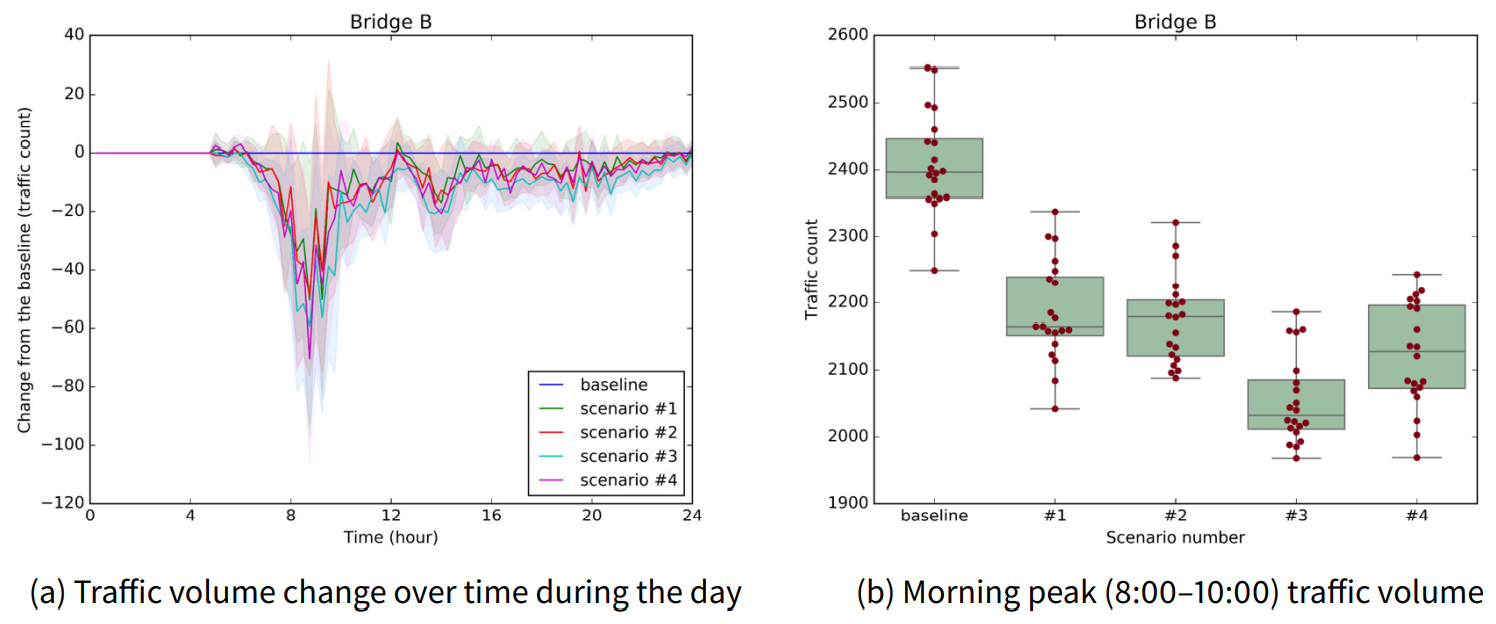
Figure 11 and Table 8 show the experimental results of the traffic dispersion effect for existing bridge B. Figure 11a plots the changes in the traffic volume of bridge B over time compared with the baseline for each construction scenario. Then, Figure 11b depicts the traffic volume comparison result at the morning peak of bridge B for the construction scenarios. Finally, Table 8 statistically verifies whether the morning peak traffic of bridges significantly differs between the scenarios.

Table 8: Tukey HSD test (FWER = 0.05, Bridge B)

Scenario (I)	Scenario (J)	Mean diff. (J-I)	Lower	Upper	p-value	Reject	Less traffic
baseline	#1	-220.65	-284.61	-156.69	0.001	True	#1
baseline	#2	-232.05	-296.01	-168.09	0.001	True	#2
baseline	#3	-353.20	-417.16	-289.24	0.001	True	#3
baseline	#4	-284.35	-348.31	-220.39	0.001	True	#4
#1	#2	-11.4	-75.36	52.56	0.9	False	-
#1	#3	-132.55	-196.51	-68.60	0.001	True	#3
#1	#4	-63.70	-127.66	0.26	0.051	False	-
#2	#3	-121.15	-185.11	-57.19	0.001	True	#3
#2	#4	-52.30	-116.26	11.66	0.1625	False	-
#3	#4	68.85	4.89	132.81	0.028	True	#3

We modeled ten types of population agent behavior: sleep, rest at home,

The result of bridge B provides similar implications for the case of bridge A. As the location of the new bridge approaches bridge B, the traffic dispersion effect of the new bridge on bridge B increases (until scenario #3), and when the new bridge is too close to bridge B, the dispersion effect decreases (in scenario #4). The difference between the results of bridge B and the results of bridge A is the optimal point. For bridge B, scenario #3 is a statistically significant best candidate in terms of traffic dispersion. Meanwhile, for bridge A, the traffic dispersion effect of scenarios #2 and #3 are not statistically significantly different.

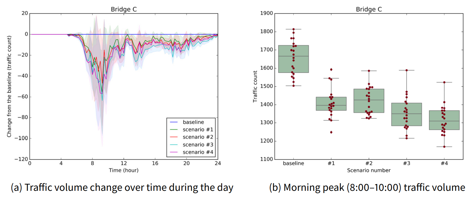
Figure 12 and Table 9 show the traffic volume comparison results for the bridge construction scenarios for bridge C. Unlike the previous cases of bridge A and bridge B, we find that the traffic dispersion effect monotonically increases as the location of the new bridge approaches bridge C. Although there is no statistically significant difference between the adjacent scenarios, the mean of the traffic volume gets smaller as the new bridge location moves to the left. In addition, in the case of scenario #4, the new bridge has a statistically significantly larger traffic dispersion effect compared with the cases of scenarios #1 and #2.

Table 9: Tukey HSD test (FWER = 0.05, Bridge C)

Scenario (I)	Scenario (J)	Mean diff. (J-I)	Lower	Upper	p-value	Reject	Less traffic
baseline	#1	-250.00	-324.40	-175.60	0.001	True	#1
baseline	#2	-237.00	-311.40	-162.60	0.001	True	#2
baseline	#3	-303.25	-377.65	-228.85	0.001	True	#3
baseline	#4	-341.60	-416.00	-267.20	0.001	True	#4
#1	#2	13.00	-61.40	87.40	0.9	False	-
#1	#3	-53.25	-127.65	21.15	0.279	False	-
#1	#4	-91.60	-166.00	-17.20	0.008	True	#4
#2	#3	-66.25	-140.65	8.15	0.105	False	-
#2	#4	-104.60	-179.00	-30.20	0.002	True	#4
#3	#4	-38.35	-112.75	36.053	0.594	False	-

Finally, Figure 13 and Table 10 show the results of the traffic dispersion experiment for bridge D. Different from the other existing bridges (A, B, and C), the location of bridge D is on the right side. Except for in the case of the direction, bridge D’s results show a similar pattern to the results of bridge C. From the results of bridge D, we find a monotone increasing pattern between the inter-bridge distance and the traffic dispersion effect. As the location of the new bridge is closer to bridge D, the new bridge’s traffic-reducing effect on bridge D increases.

Table 10: Tukey HSD test (FWER = 0.05, Bridge D)

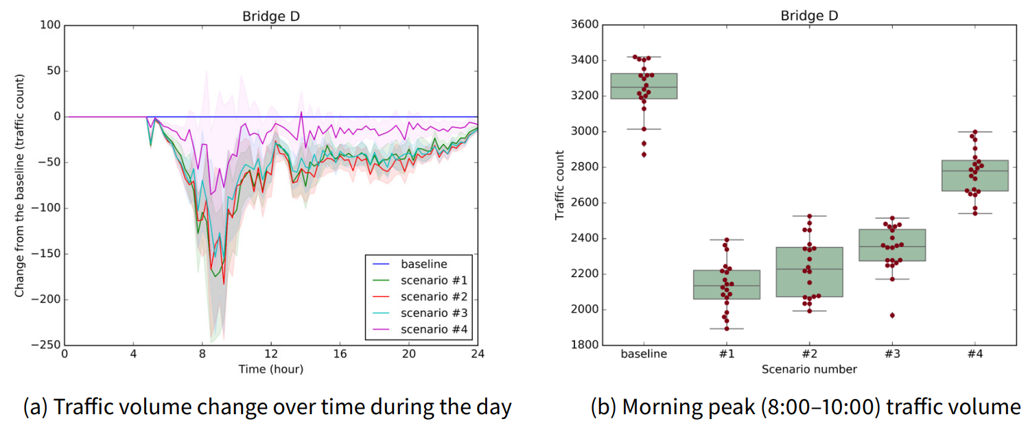
Scenario (I)	Scenario (J)	Mean diff. (J-I)	Lower	Upper	p-value	Reject	Less traffic
baseline	#1	-1097.10	-1224.69	-969.51	0.001	True	#1
baseline	#2	-996.80	-1124.39	-869.21	0.001	True	#2
baseline	#3	-895.45	-1023.04	-767.86	0.001	True	#3
baseline	#4	-464.05	-591.64	-336.46	0.001	True	#4
#1	#2	100.30	-27.29	227.89	0.194	False	-
#1	#3	201.65	74.06	329.24	0.001	True	#1
#1	#4	633.05	505.46	760.64	0.001	True	#1
#2	#3	101.35	-26.24	228.94	0.185	False	-
#2	#4	532.75	405.16	660.34	0.001	True	#2
#3	#4	431.40	303.81	558.99	0.001	True	#3

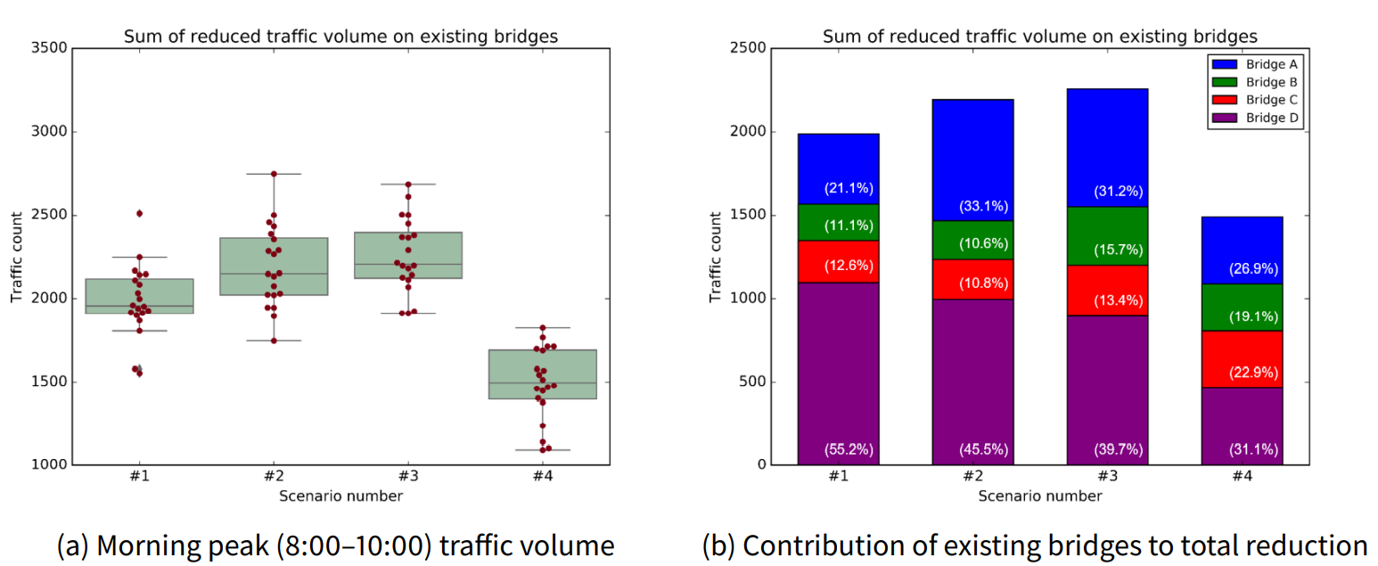
To comprehensively check the traffic volume changes of the existing bridges, we employed the sum of reduced traffic volume on existing bridges as an evaluation metric for construction scenarios. Figure 14 shows the sum of the traffic reductions of existing bridges by construction scenario and existing bridges’ contribution to the total reduction. Similar to the inverted-U shape of bridges A and B, the total traffic reduction increases as the location of the new bridge get closer to the left, and then, it decreases when moves too far.

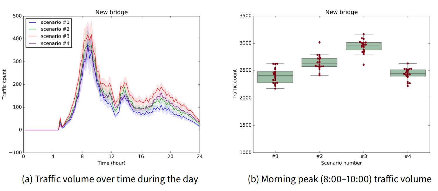
Next, we investigated the traffic volume of the new bridge, as an additional scenario evaluation metric. Figure 15 and Table 11 show the comparison results for each scenario of the new bridge traffic volume. Because the new bridge is virtual that does not currently exist, the baseline case is omitted from the figures and table related to the new bridge. Figure 15a shows the traffic volume by time of the new bridge for each scenario, and Figure 15b denotes the morning peak traffic volume of the new bridge for each scenario. Finally, Table 11 statistically compares the morning peak traffic volume of the new bridge between the location scenarios. From the results, we confirmed that the valuation of each scenario varies according to the evaluation metric. For both metrics, total traffic reduction and new bridge traffic volume, it is the same that scenario #3 is the optimal construction location. However, scenario #4 becomes the worst choice with the new bridge traffic volume metric. This implies that different evaluation metrics may lead to different decisions of policymakers.

Table 11: Tukey HSD test (FWER = 0.05, New Bridge)

Scenario (I)	Scenario (J)	Mean diff. (J-I)	Lower	Upper	p-value	Reject	More demand
#1	#2	242.40	137.38	347.42	0.001	True	#2
#1	#3	543.00	437.98	648.02	0.001	True	#3
#1	#4	29.25	-75.77	134.27	0.874	False	-
#2	#3	300.60	195.58	405.62	0.001	True	#3
#2	#4	-213.15	-318.17	-108.13	0.001	True	#2
#3	#4	-513.75	-618.77	-408.73	0.001	True	#3

Microscopic result analysis

As the second part of the policy experiment, we analyze microlevel results to understand the cause of the non-linear relationship between inter-bridge distance and the traffic dispersion effect. The results of this part are related to the RQ2 mentioned in the introduction section. We perform the destination profiling of the population passing through the new bridge.

First, we generate destination information for the population agents passing through the new bridge at the morning peak (08:00–10:00). Then, we classified the destinations of the population in four major regions. Figure 16a plots the regional classification information as well as an example of the destination distribution on the map. Finally, we calculate the volume and the proportion of the population agents who are destined for each region. Figure 16b depicts the destination classification results for each new bridge construction scenario. The graph above shows the traffic volume information, and the graph below shows the proportion information.

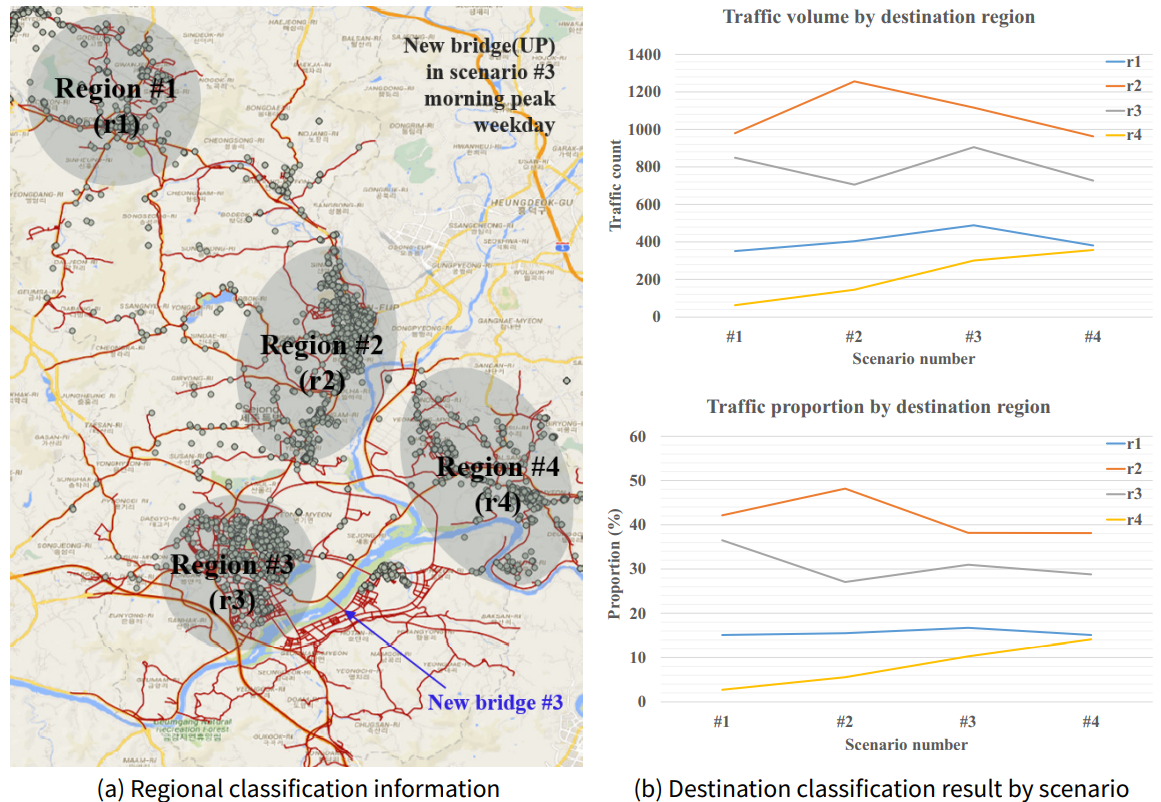
From the traffic volume result, we check to see if the preferred new bridge location is different for each population subgroup. For the population subgroups heading towards the r1 and r2 regions, the preference according to the new bridge location shows an inverted-U shape. These subgroups prefer the new bridge location to be midway between existing bridges (scenario #2 and scenario #3) rather than being adjacent to the existing bridges (scenario #1 and scenario #4). This result infers that these subgroups need a detour that is differentiated from the existing route, and therefore, they prefer that the new bridge be located away from the existing bridges.

For the population subgroup heading toward the r3 region, the preference according to the new bridge location has a more complex shape. To specify the relationship pattern between the new bridge location and the preference, we need to conduct additional simulation experiments including higher resolution location scenarios. However, among the given new bridge location scenarios, scenario #3 is the most preferred location for this subgroup. Finally, for the population subgroup heading toward the r4 region, the preference according to the new bridge location monotonically increases. For this subgroup, the preference for new bridges increases as the bridge moves to the left. This result infers that this subgroup does not require a detour differentiated from the existing route. Instead, they prefer to have new bridges located close to existing bridges to solve the traffic congestion problem on the bridges, which are the bottlenecks of the existing routes.

Discussion

In this section, we outline the limitations of the implemented model as well as future works to improve it. The first item to be discussed is the destination selection process. The destination selection process reproduces the motives of population movement. We believe that this process is the most important part of a model aimed at predicting the demand for road infrastructure or transportation. In our implemented model, we consider only two variables, the type of building and the distance from the current location, in the destination selection process. This process is quite abstract compared with reality and needs to be more complex. We summarize the points that need to be improved or added as follows.

Homogeneous utility modeling of buildings. We implement the purpose of each building heterogeneously through building-type modeling. However, we do not consider the utility of the building in the destination selection process. In other words, all buildings have the same utility. In reality, the distribution of users in restaurants or stores is not uniform, which means that the utility they provide is not the same. If we consider the utility of the building in the destination selection process as well, we believe that we can advance our model validity. We are able to estimate the utility of a building from the number of visitors or from total sales information based on card usage data.

Simple distance calculation between buildings. We use the Euclidean distance to measure the distance between buildings in the destination selection process. Our ultimate modeling goal is to use the shortest time path considering the temporal road traffic speed instead of the Euclidean distance. In the current model, decisions about individual behavior and movement influence road traffic, but there is no channel where the traffic influences the agent’s behavior. By taking the shortest time path into account in the destination selection, we are able to create a feedback loop between the agent and the road traffic. However, in the current model, we used the simple distance measure due to the expensive computation cost.

The next topic of discussion is the means of transportation. In reality, it is natural that changes in traffic infrastructure and road traffic conditions affect individual means of transportation choices. However, in our model, only walking, cars, and buses are implemented as means of transportation. Also, the means of transportation selection process considers only vehicle accessibility and distance to destination. The points required for the advancement of this process are summarized as follows.

Diversity of means of transportation. Our model mainly deals with road traffic, and we consider only private cars as road traffic. Accordingly, the current model implements only cars, buses, and walking as means of transportation. However, increasing the choice of transportation options is one factor that can reduce road traffic. In reality, there are many other means of transportation, such as taxis, bikes, and scooters. Increasing the diversity of means of transportation in the model is a further direction for advancement.

Transportation costs and demographic characteristics. In reality, transportation costs and the demographics of agents are major factors that influence transportation choice, along with distance and vehicle accessibility. Bus fares, parking lot fees, and fuel costs may be considered as examples of transportation costs. These transportation costs are introduced along with time into the agent’s utility function to model more realistic transportation selection. Also, the agent’s demographic characteristics are able to be taken into account in the transportation selection. For example, it is possible to implement the assumption that an agent with low income is more sensitive to cost changes by modifying the coefficients of the utility function. We can similarly apply these items to the advancement of the destination decision process.

The final discussion topic is parameter calibration from the perspective of output validation. We set model parameters that are difficult to observe from reality as values that best reproduce real traffic data. The parameter calibration process consists of two steps. We summarized the limitations of each step as follows.

Arbitrary setting of parameter range. First, we define the search space by setting the upper and lower limits of the calibration target parameters. It is necessary to estimate reasonable parameter ranges. For some parameters, such as those related to traffic speed estimation, we are able to determine a reasonable range of parameters using the traffic volume and traffic speed data pairs from the VDS (e.g., \(\delta_1\), \(\delta_2\), \(\delta_3\), and \(\delta_4\)). However, it is difficult to set an appropriate range for the parameters where corresponding observations cannot be obtained. Inevitably, we arbitrarily set ranges for these unobservable parameters (e.g., \(\alpha\), \(\beta\), and \(\gamma\)). We try to compensate for this contrivance by setting the search range to be wide. However, this part also needs to be replaced with data-based estimation in further works.

Robustness and convergence check. Next, we sample the parameter combinations within a given search space. Among the sampled parameter combinations, the best one in terms of the R-squared measure is selected. However, we do not check the robustness and convergence of the selected combination. We only guarantee that it is the best among the sampled combinations. By applying the gradient-based search algorithm, we expect that robustness and convergence checks for the searched parameter combinations will be possible. However, real-scale model implementation is one of the prerequisites for our study, and thus, our simulation model requires many computational resources. One simulation run takes about 40 minutes of wall-clock time on the Xeon E5-2640 CPU. It is hard to apply the machine learning-based search algorithm with our limited computational resources, so we leave it as further work.

Conclusion

In summary, our study provides the following two implications. First, it provides policy implications about the traffic dispersion effect. We find that several relationship patterns exist between the inter-bridge distance and the traffic dispersion effect (e.g., inverted-U shape, monotonically increasing shape). Although our case alone cannot make generalizations or verify the determinants of these relationship patterns. We leave this part for further works or more empirical studies.

Next, our work provides methodological implications for urban simulation. From the microscopic results, we find evidence that the preferred location of the new bridge may be different for some population subgroups, especially depending on their destinations. Considering our model components, it is self-evident that the population’s destination distribution is the result of the interaction between the population and the urban infrastructure (e.g., the population’s residence distribution, the distribution of building locations and types, the population’s behavioral patterns). In other words, for the urban simulation to provide better policy implications for administrators, it is necessary to integrate multiple distributions of the real world into a single model. The agent-based modeling framework is one way in which to unite multiple real-world distributions and to simulate their interactions, and our study provides an appropriate example of this.

References

ADELT, F., Weyer, J., Hoffmann, S., & Ihrig, A. (2018). Simulation of the governance of complex systems (SimCo): Basic concepts and experiments on urban transportation. Journal of Artificial Societies and Social Simulation, 21(2), 2; https://www.jasss.org/21/2/2.html. [doi:10.18564/jasss.3654]

ARSHAM, H., & Kahn, A. (1990). “What-if” analysis in computer simulation models: A comparative survey with some extensions. Mathematical and Computer Modelling, 14, 101–106. [doi:10.1016/0895-7177(90)90156-h]

BAE, J. W., & Moon, I.-C. (2015). LDEF formalism for agent-based model development. IEEE Transactions on Systems, Man, and Cybernetics: Systems, 46(6), 793–808. [doi:10.1109/tsmc.2015.2461178]

BAE, J. W., Shin, K., Lee, H.-R., Lee, H. J., Lee, T., Kim, C. H., Cha, W.-C., Kim, G. W., & Moon, I.-C. (2018). Evaluation of disaster response system using agent-Based model with geospatial and medical details. IEEE Transactions on Systems, Man, and Cybernetics: Systems, 48(9), 1454–1469. [doi:10.1109/tsmc.2017.2671340]

BARBROOK-JOHNSON, P., Badham, J., & Gilbert, N. (2017). Uses of agent-based modeling for health communication: The TELL ME case study. Health Communication, 32(8), 939–944. [doi:10.1080/10410236.2016.1196414]

BARDE, S., & van der Hoog, S. (2017). An empirical validation protocol for large-scale agent-based models. Bielefeld Working Papers in Economics and Management No. 04-2017. Available at: https://papers.ssrn.com/sol3/papers.cfm?abstract_id=2992473. [doi:10.2139/ssrn.2992473]

BIEKER, L., Krajzewicz, D., Morra, A., Michelacci, C., & Cartolano, F. (2015). 'Traffic simulation for all: A real world traffic scenario from the city of Bologna.' In M. Behrisch & M. Weber (Eds.), Modeling Mobility with Open Data (pp. 47–60). Berlin Heidelberg: Springer. [doi:10.1007/978-3-319-15024-6_4]

BOEL, R., & Mihaylova, L. (2006). A compositional stochastic model for real time freeway traffic simulation. Transportation Research Part B: Methodological, 40(4), 319–334. [doi:10.1016/j.trb.2005.05.001]

BRILON, W. (2000). Traffic flow analysis beyond traditional methods. Proceedings of the 4th International Symposium on Highway Capacity, Maui, Hawaii.

BROOMFIELD, H., & Reutter, L. M. (2021). Towards a data-Driven public administration: An empirical analysis of nascent phase implementation. Scandinavian Journal of Public Administration, 25(2), 73–97.

BURGHOUT, W. (2004). Hybrid microscopic-mesoscopic traffic simulation. KTH, PhD Thesis. Available at: https://www.diva-portal.org/smash/get/diva2:14700/FULLTEXT01.pdf.

CHEN, B., Sun, D., Zhou, J., Wong, W., & Ding, Z. (2020). A future intelligent traffic system with mixed autonomous vehicles and human-driven vehicles. Information Sciences, 529, 59–72. [doi:10.1016/j.ins.2020.02.009]

CHU, L., Liu, H. X., Oh, J.-S., & Recker, W. (2003). A calibration procedure for microscopic traffic simulation. Proceedings of the 2003 IEEE International Conference on Intelligent Transportation Systems, 2003, pp. 1574-1579 vol.2.

COESTER, A., Hofkes, M. W., & Papyrakis, E. (2018). Economics of renewable energy expansion and security of supply: A dynamic simulation of the German electricity market. Applied Energy, 231, 1268–1284. [doi:10.1016/j.apenergy.2018.09.143]

COLLIER, N., & North, M. (2013). Parallel agent-based simulation with repast for high performance computing. Simulation, 89(10), 1215–1235. [doi:10.1177/0037549712462620]

DELLE Monache, M. L., Chi, K., Chen, Y., Goatin, P., Han, K., Qiu, J.-M., & Piccoli, B. (2021). A three-phase fundamental diagram from three-dimensional traffic data. Axioms, 10(1), 17. [doi:10.3390/axioms10010017]

ELEFTERIADOU, L. (2014). An Introduction to Traffic Flow Theory. Berlin Heidelberg: Springer.

FAGIOLO, G., & Roventini, A. (2017). Macroeconomic policy in DSGE and agent-Based models redux: New developments and challenges ahead. Journal of Artificial Societies and Social Simulation, 20(1), 1. https://www.jasss.org/20/1/1.html. [doi:10.18564/jasss.3280]

GAO, W., Balmer, M., & Miller, E. J. (2010). Comparison of MATSim and EMME/2 on greater Toronto and Hamilton area network, Canada. Transportation Research Record, 2197(1), 118–128. [doi:10.3141/2197-14]

GE, J., & Polhill, G. (2016). Exploring the combined effect of factors influencing commuting patterns and CO2 emissions in Aberdeen using an agent-based model. Journal of Artificial Societies and Social Simulation, 19(3), 11. https://www.jasss.org/19/3/11.html. [doi:10.18564/jasss.3078]

GILBERT, N., Ahrweiler, P., Barbrook-Johnson, P., Narasimhan, K. P., & Wilkinson, H. (2018). Computational modelling of public policy: Reflections on practice. Journal of Artificial Societies and Social Simulation, 21(1), 14 : https://www.jasss.org/21/1/14.html. [doi:10.18564/jasss.3669]

HELBING, D., Hennecke, A., Shvetsov, V., & Treiber, M. (2001). MASTER: Macroscopic traffic simulation based on a gas-kinetic, non-local traffic model. Transportation Research Part B: Methodological, 35(2), 183–211. [doi:10.1016/s0191-2615(99)00047-8]

HIDAS, P. (2002). Modelling lane changing and merging in microscopic traffic simulation. Transportation Research Part C: Emerging Technologies, 10(5), 351–371. [doi:10.1016/s0968-090x(02)00026-8]

HM Treasury. (2013). The Green Book: Appraisal and evaluation in central government. Available at: https://www.gov.uk/government/publications/the-green-book-appraisal-and-evaluation-in-central-governent.

KHAN, Z. H., & Gulliver, T. A. (2018). A macroscopic traffic model for traffic flow harmonization. European Transport Research Review, 10(2), 1–12. [doi:10.1186/s12544-018-0291-y]

KIM, J., KIM, N., Paik, E., Lee, C.-H., & Bae, J. W. (2017). Practical application of wedding ring in agent-based demographic simulation. IEEE 2017 Winter Simulation Conference (WSC). [doi:10.1109/wsc.2017.8248143]

KLÜGL, F., & Bazzan, A. L. C. (2004). Route decision behaviour in a commuting scenario: Simple heuristics adaptation and effect of traffic forecast. Journal of Artificial Societies and Social Simulation, 7(1), 1. https://www.jasss.org/7/1/1.html.

KOREA Transport DB. (2019). Korea transportation network geographic information system data. Available at: https://www.ktdb.go.kr/www/contents.do?key=202.

KUMAR, S., & Mitra, S. (2006). Self-organizing traffic at a malfunctioning intersection. Journal of Artificial Societies and Social Simulation, 9(4), 3. https://www.jasss.org/9/4/3.html.

LEE, H., LEE, H.-W., & Kim, D. (2001). Macroscopic traffic models from microscopic car-following models. Physical Review E, 64(5), 056126. [doi:10.1103/physreve.64.056126]

LENGYEL, J., & Friedrich, J. (2019). Multiscale urban analysis and modelling for local and regional decision-makers. International conference on Smart and Sustainable Planning for Cities and Regions. [doi:10.1007/978-3-030-57332-4_40]

LIGHTHILL, M. J., & Whitham, G. B. (1955). On kinematic waves II. A theory of traffic flow on long crowded roads. Proceedings of the Royal Society of London. Series A. Mathematical and Physical Sciences, 229(1178), 317–345.

LU, Q., Tettamanti, T., Hörcher, D., & Varga, I. (2020). The impact of autonomous vehicles on urban traffic network capacity: An experimental analysis by microscopic traffic simulation. Transportation Letters, 12(8), 540–549. [doi:10.1080/19427867.2019.1662561]

MANSON, S. M. (2003). 'Validation and verification of multi-agent models for ecosystem management.' In M. Janssen (Ed.), Complexity and Ecosystem Management: The Theory and Practice of Multi-Agent Approaches (pp. 63–74). Northampton, MA: Edward Elgar Publishers.

MCKAY, M., Beckman, R., & Conover, W. (1979). Comparison of three methods for selecting values of input variables in the analysis of output from a computer code. Technometrics, 21(2), 239–245. [doi:10.1080/00401706.1979.10489755]

MIHĂIŢĂ, A. S., Ortiz, M. B., Camargo, M., & Cai, C. (2019). Predicting air quality by integrating a mesoscopic traffic simulation model and simplified air pollutant estimation models. International Journal of Intelligent Transportation Systems Research, 17(2), 125–141.

PATELLA, S., Scrucca, F., Asdrubali, F., & Carrese, S. (2019). Carbon footprint of autonomous vehicles at the urban mobility system level: A traffic simulation-based approach. Transportation Research Part D: Transport and Environment, 74, 189–200. [doi:10.1016/j.trd.2019.08.007]

RATROUT, N. T., & Rahman, S. M. (2009). A comparative analysis of currently used microscopic and macroscopic traffic simulation software. The Arabian Journal for Science and Engineering, 34(1B), 121–133.

RUSSELL, S., & Norvig, P. (2009). Artificial Intelligence: A Modern Approach. Hoboken, NJ: Prentice Hall.

SEJONG Public Data. (2019a). Business license data. Available at: https://www.localdata.kr/devcenter/dataDown.do?menuNo=20001.

SEJONG Public Data. (2019b). Sejong traffic information system: Bus information. Available at: https://bis.sejong.go.kr/web/main/main.view.

SINGH, K., Ahn, C.-W., Paik, E., Bae, J. W., & Lee, C.-H. (2018). A micro-level data-calibrated agent-based model: The synergy between microsimulation and agent-based modeling. Artificial Life, 24(02), 128–148. [doi:10.1162/artl_a_00260]

STATISTICS Korea. (2014). Time-use survey data: Total amount of time. Available at: https://mdis.kostat.go.kr/extract/extYearsSurvSearchNew.do?curMenuNo=UI_POR_P9012.

STATISTICS Korea. (2015). Population and housing census: 2% population data.

SUN, B., Appiah, J., & Park, B. B. (2020). Practical guidance for using mesoscopic simulation tools. Transportation Research Procedia, 48, 764–776. [doi:10.1016/j.trpro.2020.08.078]

TAYLOR, N. B. (2003). The CONTRAM dynamic traffic assignment model. Networks and Spatial Economics, 3(3), 297–322.

THONHOFER, E., Palau, T., Kuhn, A., Jakubek, S., & Kozek, M. (2018). Macroscopic traffic model for large scale urban traffic network design. Simulation Modelling Practice and Theory, 80, 32–49. [doi:10.1016/j.simpat.2017.09.007]

TUKEY, J. W. (1949). Comparing individual means in the analysis of variance. Biometrics, 5(2), 99–114. [doi:10.2307/3001913]

YUN, T.-S., & Moon, I.-C. (2020). Housing market agent-Based simulation with loan-To-Value and debt-To-Income. Journal of Artificial Societies and Social Simulation, 23(4), 5: https://www.jasss.org/23/4/5.html. [doi:10.18564/jasss.4410]

YÜCEL, G., & van Daalen, E. (2009). An objective-based perspective on assessment of model-supported policy processes. Journal of Artificial Societies and Social Simulation, 12(4), 3: https://www.jasss.org/12/4/3.html.

ZIEMKE, D., Knapen, L., & Nagel, K. (2021). Expanding the analysis scope of a matsim transport simulation by integrating the FEATHERS activity-based demand model. Procedia Computer Science, 184, 753–760. [doi:10.1016/j.procs.2021.04.022]